Chapter 13 - Experimentation
This chapter tells you all about the experimentation features in GPSS World, and how to use them. A general overview is presented in the chapter introduction, followed by background material, then a detailed presentation of all the features relating to experimentation. We conclude the chapter with a list of practical tips that address problems you may encounter.
You should be able to get started after reading the introduction if you are willing to use the Help facilities, the Tutorial Manual, and refer to details in this manual. If you are unfamiliar with some of the nomenclature you may want to read section 13.2.2 first.
However, to get to most out of what GPSS World offers you need to become familiar with what lies in the rest of this chapter. Also helpful are several new sample models including OneWay.gps, Multiway.gps, ExperEther.gps, LatinSquare.gps, GraecoLatin.gps and Lessons 19 and 20 in the Tutorial Manual.
13.1 Introduction
The experimental phase of a simulation project assumes the existence of a fully developed, well-tested, GPSS World simulation that embodies the influences of each of the factors whose effects are to be measured. Only then, should you proceed with the experimental phase of your project. Conceptually, GPSS World supports three different approaches to experimentation: Screening Experiments, User Experiments, and Optimizing Experiments. There are features that support each of these.
The Experiments generated by GPSS World use partial factorial experiments with a fixed number of treatment levels for each factor. When you create your own experiments, you do not have this restriction. You are limited to 6 factors, each of which may have any number of treatment levels. Your job then is to define a one-way or an orthogonal experiment, fill a Result Matrix with the yield of each run, and pass it to the ANOVA library procedure.
13.1.1 Screening Experiments
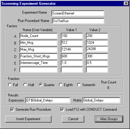
A Screening Experiment is usually used to identify the most important factors affecting the simulated system. This information is crucial for directing the rest of the investigation in the most efficient way. The results of a screening experiment show which factors are not effective and should receive low priority with respect to further study. Also, the sensitivity of the yields of an experiment to one or more of the screened factors raises a flag that assumptions made in this part of the simulation should be verified carefully. GPSS World has an automatic experiment generator that can create Screening Experiments for you. To use it, you fill in a dialog that is accessed from the Edit Menu of the Main Window. This results in PLUS code being inserted into your Model Object. Optionally, this process will also load a Function Key with the appropriate CONDUCT Command for the simulation. After that, your role is to create the Simulation Object (Ctrl+Alt+S), start the experiment (normally F11), and then analyze the results.
13.1.2 User Experiments
User Experiments are more flexible, but you must create and run them yourself. Even so, GPSS World provides a lot of support along the way. The ultimate goal is for you to provide the data needed by the GPSS World ANOVA library procedure, which will analyze your experiments with up to 6 factors, including 2 and 3-way interactions between factors. The main requirement of GPSS World ANOVA is that you must pass it the name of the GPSS Matrix where the results of your experiment have been saved.
There are two important things to know about Result Matrices. First, before you begin your experiment you should initialize your Matrix's elements to the UNSPECIFIED state. Here's a typical Statement to do this:
INITIAL MyResultMatrix,UNSPECIFIED
This makes it clear to the ANOVA routine when a run of the experiment has not been completed.
The second thing is that if your experiment has more than one factor, you need to make it symmetrical so that the GPSS World ANOVA routine can cleanly analyze the variance. The technical term for this special symmetry is "orthogonality". All you have to do to achieve orthogonality is to look at all pairs of factors in your experiment. If, within each pair, each Treatment Level of the first Factor appears the same number of times within each Treatment Level of the second Factor, the experiment will be orthogonal. If you make everything symmetrical, it will be orthogonal. Don't worry, GPSS World will tell you when it's not.
GPSS World provides the PLUS Language that you can use to write programmable experiments. A good way to get started is to look at chapters 19 and 20 in the Tutorial Manual, or to use the automatic experiment generators in the Edit Menu to create samples for you to follow. Actually, you don't really need to use PLUS. You can set up your own Command lists in Include-files or enter them manually. All you need is some way to get the yield(s) of each run in your experiment into one or more Result Matrices that can be passed to the ANOVA library procedure.
If you do decide to write your experiment in PLUS, you should consider using the same programming style as the automatic experiment generators, which is discussed later in this chapter. The use of a Run Procedure is a case in point. A Run Procedure is a simple PLUS Procedure that is called every time a run in the experiment is to be performed. Since the Run Procedure is called by a PLUS Experiment, it is permitted to invoke the DoCommand library procedure, giving it the power to issue RMULT, START, RESET, and other Commands. It is then convenient to place all the Commands needed to set up each run into the Run Procedure. To reset variables in the Run Procedure, you should use the CLEAR ,OFF form of the CLEAR Command so that your Result Matrix is preserved. To vary the Random Number seeds, generated experiments pass a unique run number as an argument to the Run Procedure. However, you may prefer to do this in some other way. One last hint: since the command string passed to the DoCommand library procedure is eventually Translated in global scope, you must avoid using local argument and temporary variable names in it. If you need to use values from arguments or temporary variables, just build the command string dynamically before invoking DoCommand, as is done in the generated experiments. This is discussed further, below, in Section 13.3.2.
13.1.3 Optimizing Experiments
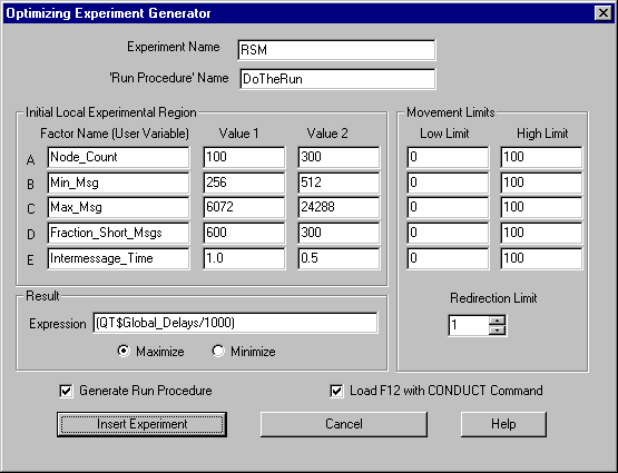
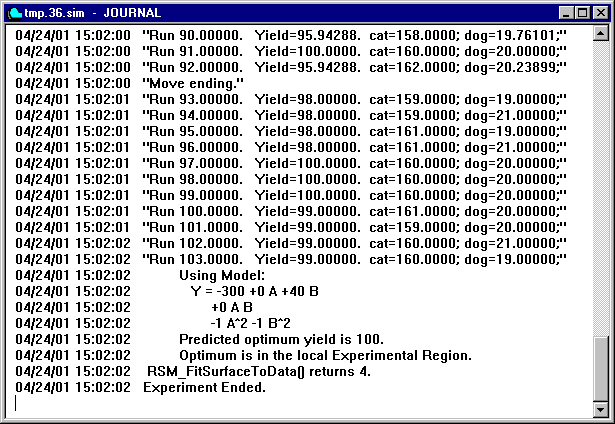
Optimization and the quantitative prediction of the behavior of a system are often the primary objectives of a simulation project. Both of these are supported directly by GPSS World. A Response Surface is an equation that predicts the results of a simulation. It is often desirable to establish a Response Surface for abbreviating results, providing a predictive methodology, quantifying the sensitivity of results to numerical inputs and other assumptions, and determining optimal treatment levels. GPSS World’s programmable Experiment feature provides the basis for a variety of Response Surface methodologies. A PLUS Experiment that calculates a Response Surface can be generated automatically, based on the input from a User Dialog. The resulting Experiment attempts to use the Method of Steepest Ascent and a Method of Local Exploration to find an optimum value. If successful, it reports the mathematical description of the best fit Response Surface and the predicted optimum conditions in the Journal Window of the Simulation Object.
As with Screening Experiments, the automatic generation of an Optimizing Experiment begins in the Edit Menu of the Main Window of GPSS World. When a Model Object is selected, you can click on Edit / Insert Experiment / Optimizing ... in order to open the dialog. After you fill in the blanks, and edit the Run Procedure, GPSS World inserts the finished PLUS Experiment into your model and optionally loads the appropriate CONDUCT Command into the F12 Function Key. Then, all you must do to start the experiment is to Create the Simulation Object (Ctrl+Alt+S) and press F12.
13.2 Experimentation and The Analysis of Variance
Next we explore some of the technical considerations that are relevant to experimentation in GPSS World. This section presents a discussion of the main issues that need to be considered when you invoke the ANOVA Procedure or when you generate an Experiment.
13.2.1 Motivation
Simulations are not completely faithful to the real world system they are intended to represent. Instead, they are merely representations intended to capture the most important behavioral characteristics of the target system.
One major difference with the real world is that simulations are perfectly repeatable. That is, if we repeat a simulation many times, we get precisely the same results every time. Such a thing is extremely unlikely in the natural sciences. In fact, it is so unnatural that we intentionally introduce variability into our simulations in order to make them look more realistic. In practice, we often find simulations in which the random variation in modeled processes, artificially introduced by us, is essential for capturing the behavior of the target system.
Another source of variability that does not occur in simulations is that due to the measurement itself. Whereas in the real world some measurement tools are very noisy and troublesome, in the simulated environment we enjoy a god-like perspective where all things are ultimately knowable without disturbing the measured environment. The point is that the observations from simulations are unnaturally crisp, and may occasionally reveal effects that exist in the real world but are extremely difficult to observe there.
Unlike experiments conducted in the real world, in simulation we have much better control over the variability introduced to mimic the apparent randomness of repeated real world measurements. Generally, we introduce one or more streams of "pseudo" random numbers, which are able to pass certain statistical tests of randomness. We go even further when we select probability distributions thought to accurately reflect the target system’s behavior. GPSS World provides over twenty of these, to be selected and used by the simulation analyst. In our quantitative analysis of simulation results, we will assume we have successfully modeled the random variance of measured values in the real world in this way.
The Analysis of Variance, or ANOVA, is a highly developed methodology for extracting information from the results of an experiment. In essence, it breaks up the variance of observations, and associates the pieces with the experimental factors and their interactions. One part, called the Error term, is associated with the unavoidable intrinsic randomness of the observations. In one sense, ANOVA attempts to account for all the variation of the observations from their average. That which is left over, the "Error", is a variation that has not been accounted for by association with the experimental conditions. It is an estimate of the intrinsic variability of observations called the Standard Error. Usually, only those effects that exceed the magnitude of the Standard Error are presumed to be real and not due to random fluctuations. A test using the "F Statistic" is normally used to ascertain this.
We must be careful to distinguish the variance introduced for realism from the variance encountered in our statistical models, the Standard Error. Generally, we do not want to distort the former because it will often cause our simulation to miss important real world behavior. On the other hand, the purpose of Design of Experiments is to reduce the unaccounted variance in our statistical analysis. This is quite a different matter. Variance Reduction Techniques, which distort variance introduced for realism, are to be avoided in the methodology we are presenting here. Our goal is to model real-world randomness accurately, not to reduce it.
We are, however, motivated to find ways to reduce the variability of the observations in the Analysis of Variance, as long as we do not distort the way we represent natural randomness. Reducing the estimate of the Standard Error in an Analysis of Variance allows significant effects to emerge above the statistical noise level. Two methods of doing so, which we will discuss below, improve the residual data used in the estimate of the Standard Error. The first by increasing the number of observations, the second by changing the underlying statistical model. These are discussed in Section 13.2.3.
13.2.2 Nomenclature
When we conduct an experiment we begin by selecting one or more metrics that quantify the state of the system or some other outcome of interest. Measurements of these quantities are called "observations" or "yields", and the set of all observations comprises the "results" of the experiment.
We will examine one or more forces called "factors" that are believed to influence the value of some of the observations. We will assign values called "treatment levels" to the factors when we specify the conditions for each execution of the simulation. When there are multiple factors, we say that the conditions are specified by "treatment combinations", since multiple treatment levels must be specified. If the influence of some factor differs when the treatment level of some other factor is varied, we say that there is an "interaction" between the two factors. Since we will be using an additive model, when the effects of two factors together is not the sum of their separate effects, we say that there is an interaction between them. There can be distinct interactions involving any number of factors.
We will simulate the target environment multiple times calling each instance a "run". The treatment combination specifies the conditions of the run, and one or more observations form the results of the run. When the conditions of a set of runs are the same except for randomization, we say that the runs in the set are "replicates", and form a "cell" of the experiment.
In the course of the Analysis of Variance, done for you by GPSS World, the observations are partitioned into components, called "effects" which are presumed to be due to the influence of the factors and their interactions. How this partition is done depends on an underlying additive model called the "statistical model". An intrinsic random deviation causes the observations to differ slightly from the sum of effects in the statistical model. The "error term" in an observation is derived by subtracting estimates of the effects corresponding to terms in the statistical model. Since the error is the quantity left over, it is often called the "residual".
For multiway experiments, that is those with more than one factor, the Analysis of Variance in GPSS World requires that the experiment be orthogonal in order to complete the analysis. This means that the estimators within the analysis must be uncorrelated. In practice, providing the same number of runs within each treatment combination of a balanced design guarantees orthogonality.
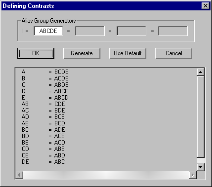
Effects, as denoted by letter groups, have important uses in the design of fractional factorial experiments, discussed below. To fractionate a factorial design, a small number of effects are chosen by the designer as "Generators" in order to specify the set of runs in the experiment. Unfortunately, this also causes some effects to become indistinguishable, or "aliased", with others. In GPSS World, the set of generators separated by equal (=) signs is called the "defining relation" of the experiment.
GPSS World supports experimentation through internal library procedures and through PLUS, the embedded Programming Language Under Simulation. PLUS is both a low-level procedural language accessible from within simulations, and a high-level control language that can direct the conditions and sequence of runs in an experiment.
13.2.3 ANOVA
The Analysis of Variance is a tool, pioneered by Sir Ronald Fisher, which is able to extract much of the information available in a set of measurements. In it, we quantify the variation of observations from the overall average, and then break it into pieces, each of which has a separate cause. If any experimental factor cannot be found to induce variability in a measurement, we say that it does not have a significant effect on it. On the other hand, if a factor does appear to induce variability, we compare the amount of it to an estimate of the intrinsic variability of the observation, the Standard Error. We do this to rule out apparent effects that are nothing more than random fluctuation. Our standard of comparison is that the variation from any source must be much larger than the Standard Error in order to be deemed a significant effect. The F test, named for Fisher, is used for this purpose. We use the F test as the criterion by which we declare the effects of experimental factors and their interactions to be statistically significant.
Implicit in the use of ANOVA is the existence of an additive mathematical model used to explain the components of variation in the observations. We will call this the "statistical model". The simplest statistical model is given in Figure 13-1.
y
i = m + eiFigure 13-1. A Simple Statistical Model
In this example, each observation is broken down into only two components, the grand mean of all observations, m, and the random component, e. Each observation has a starting point, the grand population mean, and then incurs a random deviation leading to its final value. The grand mean does not vary from observation to observation, whereas the random component does, and is subscripted accordingly. Although this model is suggestive, it allots all variation of the observations to random sources and none to factors, and so is not very useful in analyzing the results of an experiment.
Next, we turn to a statistical model used to analyze the data from an experiment with a single factor, namely, factor A.
y
i,j = m + ai + ei,j Figure 13-2. One Factor Statistical ModelIn Figure 13-2, notice the introduction of the subscripted alpha term, which denotes the effect of the ith treatment level of the one and only factor considered in the model. The experiment would include one or more runs at each of the treatment levels of factor A. All observations at a given treatment level are analyzed using the same value for a. Since there is only one factor in this experiment, the number of treatment combinations is just the number of treatment levels of that factor. An Analysis of Variance based on this statistical model will result in an ANOVA table that partitions the variation of the observations into that due to treatment A, and that due to the random variation.
y
i,j,k = m + ai + bj + i(ab)i,j + ei,j,k Figure 13-3. Two Factor Statistical ModelIn Figure 13-3, we move to a model where two factors are considered. Notice that we now include a term for the interaction between factor A and factor B, denoted i(ab). This term may differ at each treatment combination, and therefore is subscripted twice since there are two factors. Recall from above that when the effects of two factors together is not the sum of their separate effects, there is an interaction between them. The strength of the interaction between factors A and B is denoted "AB" and would be reported in a line of the ANOVA table.
In a complete factorial experiment all interaction terms would be included. Just as the complete 2-factor model in Figure 13-3 has 5 (RHS) terms, a complete 3-factor model has 8 terms, and a complete 4-factor model has 16 terms. All this information is normally presented in the resulting ANOVA table. GPSS World can handle up to 6-factor models with up to and including 3-way interactions.
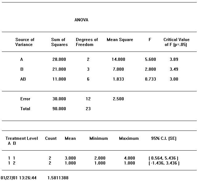
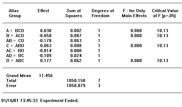
Figure 13-4, below, presents an ANOVA table reported by GPSS World. As explained above, the single capital letters denote factors and capital letter combinations denote interactions.
First, look at the bottom of the table. The Total Sum of Squares is to be partitioned, and the components are to be associated with the effects of factors and their interactions. Anything that is left over, that is, the residual sum of squares, is shown in the previous line, labeled "Error". The Mean Sum of Squares of the error term is used to estimate the Standard Error of the experiment.
Each Sum of Squares has a divisor associated with it called the Degrees of Freedom. From statistical considerations, the Degrees of Freedom is that divisor that must be used to create an unbiased estimator of the Standard Error, in the absence of other effects. For our purposes, it is sufficient to think of Degrees of Freedom as the proper divisor associated with a Sum of Squares in the ANOVA table. GPSS World will always calculate the Degrees of Freedom for you.
Figure 13-4. An ANOVA Table
Each factor and interaction in the statistical model is represented by a distinct line in the ANOVA table. In each line we have first the Sum of Squares and the Degrees of Freedom associated with that estimate. These are the basics from which the other numbers are derived. A simple division results in the Mean Square, and by dividing that quotient by the Mean Square of the Error, from the bottom row of the table, we get the F statistic for that effect.
Now we are ready to draw some conclusions. We must decide if the F value is large enough to declare that the effect is significant. The threshold value we will use to make the comparison is called the "Critical Value of F" and is placed just to the right of our F statistic on the same line. If our F value exceeds the Critical Value, we conclude that we are dealing with a significant effect. If not, we conclude that the effect is not significant and we disregard any associated variation in observations as only due to random noise. The larger the F value the stronger the effect. The ANOVA table in Figure 13-4 shows the effect of factor A to be significant and the effects from factor B and the AB interaction to be not significant.
Sometimes an experiment will fail to detect an effect even though one actually exists. One of our goals is to make this as unlikely as possible. According to the ANOVA table, there are two ways to make an experiment better able to detect real effects. To get more positive results we would need either a larger F statistic or a smaller Critical Value of F.
It is desirable to remove any part of the Sum of Squares of the Error that is due to any important effect we have not included in the analysis. If we can do this, our F statistic will generally be larger. In experimentation in the natural sciences, this is done by making comparisons in as homogenous an environment as possible, a technique known as "blocking". However, in simulation studies this goal is perhaps best approached by identifying additional factors that must be included in the experiment.
Two other approaches are directed at increasing the Degrees of Freedom of the Error term. The first is simply to increase the number of replicates in the experiment. This is usually the most expensive approach but it can be quite effective. The second possibility relates to the design of the experiment and the statistical model behind the Analysis of Variance. The Mean Square of the Error is actually a residual term left after all other squares have been removed. If we can find an acceptable way to allow more of the data to remain after the effects are removed, we will have an estimate of the Standard Error that has more degrees of freedom. The resulting Critical Value of F will be smaller, thereby increasing the power of the analysis. This is what we are attempting to do when we choose to ignore some of the interactions.
None of the techniques we are considering will distort the randomness introduced to simulate real-world randomness. Variance Reduction Techniques that do should not be used here. Intentionally reducing the intrinsic variability of the observations would cause the F statistics to be overstated.
In many multifactor experiments we will chose to remove the highest order interactions in order to improve the information available on the main factors and the low order interactions. You can do this using the third argument of the ANOVA Procedure. If it is true that these interaction effects do not exist, this will allow GPSS World to use the extra degrees of freedom to achieve a better estimate of the F statistic. In addition, more Degrees of Freedom means a smaller critical value of F, as well. However, we must realize that removing terms from the statistical model assumes that there is no high-order effect. If there is a reasonable chance of one, we would be better off adding replicates to improve the statistics rather than limiting the analysis to low order interactions. Replicates are made known to the ANOVA Procedure in its second argument.
y
i,j,k = m + ai + bj + ei,j,kFigure 13-5. Two Factor Statistical Model without Interactions
Figure 13-5 shows a statistical model in which the 2-way interaction term was removed. If it is true that the interaction effect does not exist, we have improved the crispness of the Analysis of Variance by providing more Degrees of Freedom for the Mean Square of the Error. When you choose to apply this technique, you simply change the 3rd argument of the call to the GPSS World ANOVA library procedure to remove higher order interactions from the analysis. This built-in procedure can handle up to 3-way interactions, and allows you to give up 2-way or 3-way interactions, and above, to improve the significance testing of the other effects.
13.2.4 Selecting Factors
When you use the ANOVA library procedure you must define a GPSS Matrix Entity, called the Result Matrix, to store the individual results of each run. If you were analyzing more than one metric, you would have more than one Result Matrix. Since GPSS World Matrix Entities can have up to 6 dimensions, each of any size, the Result Matrix is also limited to 6 dimensions.
When you write your own GPSS World Experiment, the most important decision you will make is to select the factors of the experiment. These are the quantities that you can control in order to optimize your system. Each factor is to be represented by a User Variable that takes on treatment levels as values. After you run each simulation in the experiment, you must place the resulting value into a Results Matrix so that the data can be analyzed by the ANOVA Procedure.
The position in the Result Matrix for each result is determined by the treatment combination. For example, if the experiment considers 4 machine types and two speeds of each, the result of simulating the third machine at high speed would go into the Result Matrix at position [3,2]. Actually, since replicates are usually tagged onto the end, the first run at this treatment combination would go into element [3,2,1] of the Result Matrix. Each dimension of the Result Matrix is analyzed as a factor by the ANOVA library procedure. The size of the dimension in the Result Matrix must be at least as large as the number the treatment levels of that factor, or of the maximum replicate count.. There is no arbitrary limit to the number of treatment levels within a factor, only that imposed by the virtual memory of your computer.
We can examine any effect by giving it it’s own dimension in the Result Matrix. If we so desire, we could even separate random number streams and treat them individually as distinct factors. Each random number seed would represent a distinct treatment level. This would provide information on the relative importance of each random input process. Usually, though, we use a single dimension for replicates, and vary all seeds from one replicate to the next within a single treatment combination. We then make known to the ANOVA Procedure which dimension is used for replicates. This is done in the second argument.
Not all experiments need a Replicate Dimension. The ANOVA is often able to extract an estimate of the Standard Error without one. The Latin Square sample model, "Latin Square.gps" is an example of this. However, depending on the design of the experiment, sometimes there is not enough residual data to estimate the Standard Error. Then the Analysis of Variance will not be able to calculate F statistics for the ANOVA Table. In such cases, you will have to either add replicate runs to the experiment or remove high level interactions from the statistical model in order to provide enough residual data for the estimate of the Standard Error. Both of these methods require a change in the call to the ANOVA library procedure.
13.2.5 The Random Number Streams
A guideline often used in the design of experiments is this: control all factors that you can; what you can’t control, block; what you can’t block, randomize. This applies to the use of the random streams in a discrete event simulation, as well.
To treat random number streams as factors is to allocate a dimension for each stream, and to use each distinct seed as a treatment level. Although it is possible to view the random number streams as factors in this way, and to examine their relative effects, it may be best done as a separate study. For the mainstream investigation of the main effects and interactions, we are more interested in using our random number streams to represent sources of natural and unavoidable variability, reserving the dimensions of the Result Matrix for the factors being studied.
The most common approach combines all random number streams into a single pseudo-factor, where each treatment level is a set of distinct seeds for all random number streams. A single dimension, the Replicate Dimension, is then allocated from the Result Matrix for this purpose and is made known to the ANOVA library procedure. This has some similarities with blocking, where all comparisons are performed within each homogeneous environment. The ANOVA library procedure can then treat this Replicate Dimension separately to better estimate the Standard Error of the experiment. The experiment then consists of an experimental "cell" for each treatment combination, with several replicate runs within each cell.
If these approaches are too expensive, or there isn’t a dimension to spare in the Result Matrix, the runs should be "completely randomized". This means that randomization should not be restricted in any way, and that the random number seeds should not be repeated within a single random number stream. If this procedure fails to provide enough Degrees of Freedom for the analysis, you may need to limit the level of interactions to be included in the statistical model, as well.
13.3 GPSS World Features
We turn now to the to the specific features of GPSS World which can be used in any of the experimentation phases of a simulation project. First, we consider the features provided for the analysis of User Experiments. GPSS World provides for two kinds of automatically generated experiments that are designed for you, and User Experiments that are designed by you.
13.3.1 User Experiments
The immediate goal of a User Experiment is to provide the information needed by the built-in ANOVA library procedure. That means that you must fill a Result Matrix with all the results of the experiment. If you prefer, you can do this directly through the use of Command Lists and manual entries. However, the PLUS Language, which allows you to write programmable experiments can make your life a lot easier if your experiment is complex.
You should begin by selecting the factors whose effects you will be studying. For example, you may want to measure the effect of the number of phone lines on the average waiting time in a telephone exchange. Factor A of your experiment would be the number of phone lines, and you would assign it to the first dimension of your Result Matrix. Next we decide how many treatment levels (i.e. number of phone lines) will be studied. Let's say that we want to simulate exchanges with 4, 8, and 16 lines. We would then need 3 slots in the Result Matrix for these three conditions. Therefore the first dimension in the Result Matrix would have a size of 3.
We continue to add factors to the experiment in this way, using the number of treatment levels as the size of the corresponding dimension in the Result Matrix. Normally, we use the last dimension for replicates. The size of the Replicate Dimension must obviously be large enough to contain the results from any cell (i.e. treatment combination) in the experiment. The only restriction is that the total number of dimensions cannot exceed 6. When you analyze the data, you must explicitly tell the ANOVA routine which dimension is used for replicates.
Remember to initialize the Result Matrix to UNSPECIFIED, before you begin storing results into it. That way, it is clear to the ANOVA routine when a run has not been performed.
When you call the ANOVA routine with your results, you must also decide if you want to exclude 3-way, or even 2-way, interactions from the analysis. If you can justifiably do this, you will improve the statistics in the ANOVA table.
That is a rough outline of the creation of User Experiments. In the remainder of this section we will look at the steps in more detail. We will consider the embedded PLUS programming language, the requirements and restrictions of the Result Matrix, and the use of the ANOVA library procedure. Lesson 19 of the GPSS World Tutorial Manual guides you through an example.
Experiments created using the automatic experiment generators are not considered User Experiments, and are discussed later. However, you may find it useful to study the programming of a generated experiment before you attempt to do it yourself.
13.3.2 PLUS Experiments
PLUS is a simple but powerful programming language that is an important part of the GPSS World simulation environment. It began as a source of custom programmable subroutines to be accessed during GPSS simulations, and has progressed to become a control language that can direct the details of the runs in an experiment, and report on the results. The complete description of PLUS is in Chapter 8 of this manual. Lesson 17 of the GPSS World Tutorial Manual covers it, as well.
An Experiment is a PLUS Procedure where the keyword PROCEDURE is replaced by the keyword EXPERIMENT. Experiments can do everything that normal Procedures can, and a whole lot more. An Experiment is invoked by a CONDUCT Command which names the invoked Experiment and passes it any arguments it might require.
The power of a PLUS Experiment is based on its ability to invoke the "DoCommand" library procedure. Nearly all GPSS Commands can be executed by a DoCommand invocation with a Command String as an argument. Not only can an Experiment invoke DoCommand, but also so can any normal PLUS Procedure that has been called during the execution of an Experiment. This adds a lot of flexibility to the programming of complex experiments.
An example of a DoCommand invocation is:
DoCommand("START 1000");
The DoCommand Library Function is peculiar in that its argument string is compiled in global scope. This means that you cannot reference local variables in an argument of a DoCommand invocation. Instead, if you need to pass local values to DoCommand, you must use PLUS string commands to create an argument string including evaluated results. As an example of this, here's the "Run Execution Procedure" created by the Automatic Experiment Generators to log run information to the Journal:
*******************************************************
* The Run Execution Procedure *
*******************************************************
PROCEDURE SEM_GetResult() BEGIN
/* Run Simulation and Log Results. */
/* Treatments have already been set for this run. */
TEMPORARY CurrentYield,ShowString,CommandString;
/* Run Procedure Call */
RunProc(SEM_NextRunNumber);
/* Place Run Results in Journal. */
ShowString = PolyCatenate("Run ",String(SEM_NextRunNumber),". ", "" );
ShowString = PolyCatenate(ShowString," Yield=",String(CurrentYield),". ");
ShowString = PolyCatenate(ShowString," Factor1=",String(Factor1), ";" );
ShowString = PolyCatenate(ShowString," Factor2=",String(Factor2), ";" );
ShowString = PolyCatenate(ShowString," Factor3=",String(Factor3), ";" );
CommandString = PolyCatenate("SHOW """,ShowString,"""", "" );
DoCommand(CommandString);
SEM_NextRunNumber = SEM_NextRunNumber + 1;
RETURN CurrentYield;
END;
Figure 13-6. Using a DoCommand in a PLUS Procedure
This procedure issues a SHOW Command in 3 steps. It records the result and conditions of the run in the Journal. First it creates a temporary string, ShowString, which contains variables evaluated locally. Second, it builds the overall string with the completed SHOW Command in the temporary variable CommandString. Finally, it invokes the DoCommand library procedure. Normal Procedures such as this can only invoke DoCommand when a CONDUCT Command is in effect. In other words, such Procedures must be called either directly, or indirectly, by a PLUS Experiment.
In experiments with many runs, it is convenient to use a PLUS Procedure to do the set up of each simulation run in the experiment. Such a procedure initializes the random number generators and issues commands that control the simulation. Then, you can set up your high level PLUS Experiment to call the Run Procedure each time a simulation is to be run.
An example of the default Run Procedure created by the Experiment Generators is in Section 13.4. 2. Even when GPSS World Creates the Experiment for you, it is up to you to modify the Run Procedure to fit the run conditions of your own simulation project.
13.3.3 The Result Matrix
The primary source of information from an experiment is kept in the Result Matrix. In order for the ANOVA library procedure to analyze the results of an Experiment, you must assure that the Result Matrix has been set up appropriately.
In GPSS World, a Matrix Entity can have up to 6 dimensions. There is no arbitrary limit on the size of each dimension other than that imposed by the virtual memory of the computer. However, one of the most important jobs in setting up a GPSS World Experiment is the selection of factors. Each factor to be included in the Experiment is assigned to one of the dimensions of the Result Matrix. In addition, depending on the design of the experiment, you will probably want to use one dimension for replicates, which must be large enough to handle the runs in the largest cell. For each dimension used for a factor, the size at least as large as the number the treatment levels of that factor. That is because there must be a place in the Result Matrix for each run. There can be any number of these treatments up to the limits imposed by the virtual memory of your computer.
If your experiment has more than one result metric, you need only define a separate Result Matrix for each one, and then utilize the ANOVA Procedure for each.
Viewing a Result Matrix
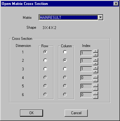
GPSS World Matrices can be viewed in a Matrix Window or printed in a Standard Report. Since GPSS World is unable to view all 6 dimensions at one time, it presents only a two dimensional slice in a Matrix Window. A small Dialogue Box is used to select the slice of the Matrix that is to appear.
Figure 13-7. The Matrix Cross Section Selection Dialog
Figure 7 presents the dialog that allows the selection of a slice through a higher order Matrix Entity. In this case we have a 3 by 4 by 2 3-dimensional Result Matrix. To use it, first select the two dimensions to form the Rows and Columns of the Matrix Window, then use the index of the remaining dimensions to select deeper slices, other than the first. It may be helpful to think of a loaf of bread seen head-on. The row and column numbers indicate where on the slice we are, and the index of the third dimension chooses the slice. In Matrices with 4 or more dimensions, an index value would be needed for each dimension not participating as a row or column.
Once the Matrix Window, itself, is open you will have the chance to scroll to any location within that slice. Matrix Windows are updated dynamically, and any number of Matrix Windows can be open at the same time.
The other way to view the elements of a Matrix Entity is to include the results in the Standard Report. Page 2 of the Settings of a Model or Simulation Object ( Edit / Settings ) has a checkbox which when checked, puts a line for each element of the Matrix in subsequent Standard Reports.
Initialization of a Result Matrix
