21. SHIPPORT.GPS
Simulation of a port.
Problem Statement
A harbor port has three berths 1, 2 and 3. At any given time Berth1 can accommodate two small ships, or one medium ship. Berth2 and Berth3 can each handle one large ship, two medium ships or four small ships.The interarrival time of ships is 26 hours, exponentially distributed, and small, medium, and large ships are in the proportions 5:3:2 respectively. Queuing for berths is on a first come first served basis, except that no medium or small ship may go to a berth for which a large ship is waiting, and medium ships have a higher priority than small ships.
Unloading times for ships are exponentially distributed with mean times as follows: small ships, 15 hours; medium ships, 30 hours; and large ships, 45 hours. The loading times are as follows:
·
Small ships 24±6 hours uniformly distributed.·
Medium ships 36±10 hours uniformly distributed.·
Large ships 56±12 hours uniformly distributed.The tide must be high for large ships to enter or leave Berths 2 and 3. Low tide lasts 3 hours, high tide, 10 hours.
1. Run the simulation for 500 days.
2. Determine the distribution of transit times of each type of ship.
3. Determine the utilization of the three berths.
Listing
; GPSS World Sample File - SHIPPORT.GPS
; Based on a model by Gerard F. Cummings
**********************************************************************
* *
* Ship and Port Simulation *
* Time in in Hours *
**********************************************************************
Berth1 EQU 1
Berth2 EQU 2
Berth3 EQU 3
Tide EQU 1
Tsmall EQU 1
Tmedium EQU 2
Tlarge EQU 3
*
*———Boolean Variables———————————————————————
Var1 BVARIABLE (R$Berth2’GE’1+R$Berth3’GE’1)#Q3’E’0
Var2 BVARIABLE R$Berth2’GE’1
Var3 BVARIABLE R$Berth3’GE’1
Var4 BVARIABLE SE$Berth1
Var5 BVARIABLE (R$Berth2’GE’2+R$Berth3’GE’2)#Q3’E’0
Var6 BVARIABLE R$Berth2’GE’2
Var7 BVARIABLE R$Berth3’GE’2
Var8 BVARIABLE SE$Berth3#LS1
Var9 BVARIABLE SE$Berth2#LS1
*
*—Size of Berths in relation to small ships—————————————
Berth1 STORAGE 2
Berth2 STORAGE 4
Berth3 STORAGE 4
*
*————Table Definations——————————————————————
Tsmall TABLE M1,30,10,20 ;Small ship transit time
Tmedium TABLE M1,30,10,20 ;Medium ship transit time
Tlarge TABLE M1,30,10,20 ;Large ship transit time
**********************************************************************
*
*————Day Timer——————————————————————————
GENERATE 24 ;One xact each day
TERMINATE 1 ;Clock operates once/day
**********************************************************************
*
*————Tide Control————————————————————————
GENERATE ,,0,1
Again LOGIC R Tide ;Cycling xact models the tide
ADVANCE 3 ;Tide is low for 3 hours
LOGIC S Tide ;Tide comes in
ADVANCE 10 ;Tide is high for 10 hrs
TRANSFER ,Again ;Branch back to ‘Again’
**********************************************************************
GENERATE (Exponential(1,0,26)) ;A ship every 26 hrs.
TRANSFER 500,,Inter ;50 % are small
*
*———Characteristics of small ships are assigned to parameters——
ASSIGN Size,1 ;Type ship small, size=1
ASSIGN Capacity,1 ;Capacity P2=1 Small ship
ASSIGN Quenum,1 ;Queue #1 for small ships
ASSIGN M_Unload,15 ;Mean unload time
ASSIGN M_Load,24 ;Mean load time
ASSIGN Loadsp,6 ;Load time spread
QUEUE P$Quenum ;Join queue-small ships
TRANSFER Both,Pier1,Pier2
*———Assign Berth 1 When Available————————————————
Pier1 GATE SNF Berth1
ASSIGN Berth_Num,1 ;Berth obtained=Berth1
*———Move into Berth and Unload and Load—————————————
Small ENTER P$Berth_num,P$Capacity ;Enter berth using up
; ship capacity
DEPART P$Quenum ;Depart queue
ADVANCE P$M_Unload,(Exponential(1,0,1)) ;Unload time
ADVANCE P$M_Load,P$Loadsp ;Loading time
TEST E P$Size,3,Skipit ;A large ship?
*———When Switch is Set, Tide is High———————————————
GATE LS Tide ;Wait for tide
Skipit LEAVE P$Berth_Num,P$Capacity ;Leave berth by
; ship capacity
TABULATE P$Quenum ;Tabulate transit time
; by ship type
TERMINATE ;Ship sails
**********************************************************************
*———Assign Berth 2 or Berth 3 when available(dependent——————
* on the ship configuration
Pier2 TEST E BV$Var1,1 ;Small ship tries 2 or 3
TRANSFER Both,Bert2,Bert3 ;Try berth2 or berth3
Bert2 TEST E BV$VAR2,1 ;Berth2 available?
ASSIGN Berth_Num,2 ;Assigned to berth2
TRANSFER ,Small
Bert3 TEST E BV$Var3,1 ;Berth3 available?
ASSIGN Berth_Num,3 ;Assigned to berth3
TRANSFER ,Small
*
*———Characteristics of medium ships are assigned to parameters——
Inter TRANSFER 400,,Large ;20% of all ships
; are large
PRIORITY 2 ;All medium ships
; enter here
ASSIGN Size,2 ;Type ship medium,
; Size=2
ASSIGN Capacity,2 ;Capacity = 2
; Medium ship
ASSIGN Quenum,2 ;Queue 2 for med ships
ASSIGN M_Unload,30 ;Mean unload time
ASSIGN M_Load,36 ;Mean load time
ASSIGN Loadsp,10 ;Load time spread
QUEUE P$Quenum ;Join queue for small
; ships
TRANSFER Both,Quay1,Quay2
Quay1 TEST E BV$Var4,1 ;Try for berth1
ASSIGN Berth_Num,1 ;Assigned to berth1
TRANSFER ,Small ;Transfer for processing
Quay2 TEST E BV$Var5,1 ;Try for berth 2 or 3
TRANSFER Both,,Quay3 ;Try berth2 first
TEST E BV$Var6,1 ;Is berth2 available?
ASSIGN Berth_Num,2 ;Gets berth2
TRANSFER ,Small ;Transfer for processing
Quay3 TEST E BV$Var7,1 ;Try for berth3
ASSIGN Berth_Num,3 ;Assigned to berth3
TRANSFER ,Small ;Transfer for
; unload/load
*
*———Characteristics of large ships are assigned to parameters——
Large PRIORITY 3 ;All large ships
; enter here
ASSIGN Size,3 ;Type ship large, Size=3
ASSIGN Capacity,4 ;Capacity=4 Large ship
ASSIGN Quenum,3 ;Queue number 3 for
; large ships
ASSIGN M_Unload,45 ;Mean unload time
ASSIGN M_Load,56 ;Mean load time
ASSIGN Loadsp,12 ;Load time spread
QUEUE P$Quenum ;Join queue for
; large ships
TRANSFER Both,First,Second ;Try Berth3 and Berth2
First TEST E BV$Var8,1 ;Try Berth3 first
ASSIGN Berth_Num,3 ;Berth number=3
; Entered Berth3
TRANSFER ,Small ;Transfer for
; unload/load
Second TEST E BV$Var9,1 ;Try berth2 second
ASSIGN Berth_Num,2 ;Berth number=2
; Entered Berth2
TRANSFER ,Small ;Transfer for
; unload/load
**********************************************************************
The model is organized into several segments. After the non-Block Entities are defined, there are three more model segments. Transactions in the top segment time the simulation and decrement the Termination Count once per simulated day. A single transaction circulates in the middle segment to represent the ebb and flow of the tides. This affects the accessibility of the berths. Transactions in the bottom segment represent ships. Each is given attributes according to the size of the ship it represents. It then waits for a suitable berth, exchanges cargo, and leaves the port.
There are 9 Boolean variables, or GPSS Bvariable Entities, defined in the beginning of the model. Boolean Variables return a value of 1 or 0 when evaluated. When the value of the BVARIABLE expression is 0 a 0 result is returned, otherwise a value of 1 is returned. They are used to determine the state of the port and which actions are possible.
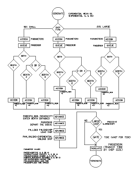
The logic of the SHIPPORT.GPS model is depicted below.
Figure 21—1. The Logic of the Shipport Model.
Running the Simulation
To run the simulation and create a Standard Report,
CHOOSE File / Open
and in the dialog box
SELECT Shipport
and then
SELECT Open
Next, create the simulation
CHOOSE Command / Create Simulation
then
CHOOSE Command / START
and in the dialog box, replace the 1.
TYPE
500SELECT OK
The simulation will end when 500 transactions have entered the TERMINATE 1 Block. This represents 500 days of operation.
When the simulation ends, GPSS World writes a report to the default report file, Shipport.1.1. As discussed in Chapter 1, the Report extension will vary depending on saved simulations and previously existing reports. For our purposes, we will assume that this is the first time the simulation has been created and run giving an extension of 1.1.
This report will be automatically displayed in a window. If you close the window, you can reopen it by using the GPSS World File / Open in the Main Menu. Then you should choose Report in the "Files of type" drop down box at the bottom of the window. GPSS World reports are written in a special format. If you wish to edit the report, you will have to copy its contents to the clipboard and from there into a word processor. You will not be able to open the file directly in a word processor.
Discussion of Results
From the GPSS Tables named "Tsmall", "Tmedium" and "Tlarge" we see histograms of the transit times for small, medium, and large ships, respectively. The average transit times were about 44, 74, and 115 hours.
The Berth utilizations were 52%, 49% and 54% for Berths 1, 2, and 3, respectively.
Inside the Simulation
Let 's now explore the ending condition of the simulation, which generated the Standard Report above. If you are not at the end of the simulation, please Retranslate the model and run it again.
Now, let’s open some graphics windows.
CHOOSE Window / Simulation Window / Storages Window
This is the Storages Window. It gives utilization and queuing information on the Berths. Notice how the color of the icons corresponds to the amount of Storage in use. Look at the histograms of transit times for small, medium, and large ships one after the other. First, for the small ships,
CHOOSE Window / Simulation Window / Table Window
and in the drop-down box in the dialog box
CLICK ON The Down Arrow at the Right End of the Box
CLICK ON TSMALL
SELECT OK
and for the medium ships
CHOOSE Window / Simulation Window / Table Window
and in the drop-down box in the dialog box
CLICK ON The Down Arrow at the Right End of the Box
CLICK ON TMEDIUM
SELECT OK
and for the large ships
CHOOSE Window / Simulation Window / Table Window
and since TLARGE is already selected in the drop-down box in the dialog box
SELECT OK
Please feel free to modify the parameters and Blocks of this simulation.
When you are done, if you wish to go on to the next lesson, close all windows related to this model.
CLICK ON The X-Upper Right of Each Window
Otherwise, to end the session
CLICK ON The X-Upper Right of Main Window.
Simulation of a PBX.
Problem Statement
A private automatic branch exchange telephone system has 200 extensions, 30 internal lines, and 30 external lines, 8 signaling units and one operator. Telephone calls last 150 seconds on average, normally distributed with a standard deviation of 30 seconds. The interarrival time of external calls varies inversely with the number of extensions (2500/number of extensions ), exponentially distributed. The interarrival time of internal calls is inversely proportional to the number of free extensions (1260/number of free extensions + 1). The destination of these calls may be internal (66.6%) or external (33.3%). The operator is not required for calls which originate internally. A signaling unit, and an internal line is required for internal calls, and an external line for external calls.Fifteen percent of extensions are engaged when tried, and twenty percent are not answered.
The time required to signal is 7±2 seconds, and to ring through to an extension is 6±2 seconds. A caller waits 4±1 seconds to check an engaged tone. The service of an operator takes 9±3 seconds.
Simulate the operation of the private branch exchange telephone system for 1 hour.
1. Determine the utilization of the operator, signaling units, internal and external lines, and the extensions.
2. Sample the number of internal and external calls being processed every minute.
3. Are the number of internal and external lines, and signaling units sufficient?
Listing
; GPSS World Sample File -
EXCHANGE.GPS, by Gerard F. Cummings
**********************************************************************
* PBX Telephone System Model
* Time is in seconds
**********************************************************************
Transit TABLE M1,20,20,20
**********************************************************************
Extensions STORAGE 200
Extlines STORAGE 30
Intlines STORAGE 30
Signals STORAGE 8
Operator STORAGE 1
**********************************************************************
* Define variables
Internal VARIABLE 1260/(1+R$Extensions)
External VARIABLE 2500/(R$Extensions+S$Extensions)
*
*Tables for number of calls in progress
Callsint TABLE S$Intlines,2,2,20
Callsext TABLE S$Extlines,2,2,20
**********************************************************************
* Generate calls originating internally
GENERATE (Exponential(1,0,V$Internal)),0,20 ;Calls origin
; internal
ENTER Extensions
;An extension is involved
QUEUE Inside
;Queue for signal unit
ENTER Signals
;Get a signaling unit
DEPART Inside
;Leave the queue
ADVANCE 7,2
;Time to signal
LEAVE Signals
;Leave the signal unit
TRANSFER .333,,Intout ;33% are internal to ext
*
Intint TEST GE R$Intlines,1,Breakoff ;Test int line available
ENTER Intlines
;Get and internal line
ADVANCE 4,1
;Check if engaged
TRANSFER .15,,Busy
;Some extensions engaged
Aline ENTER Extensions ;Another extension involved
ADVANCE 6,2
;Time to ring extension
TRANSFER .2,,Nogood
;20% not answered
ADVANCE (Normal(2,150,30)) ;Call duration
Nogood LEAVE Extensions ;Leave extension
Busy LEAVE Intlines
;Leave internal line
TRANSFER ,Breakoff
***********************************************************************
"
* Model internal to external calls
Intout TEST GE R$Extlines,1,Breakoff ;Is an ext line available?
ENTER Extlines
;Get an external line
ADVANCE 4,1
;Time to check if engaged
TRANSFER .200,,Nobody ;20% are engaged
ADVANCE 6,2
;Time to answer
TRANSFER .200,,Nobody ;20% do not answer
ADVANCE (Normal(2,150,30)) ;Call duration
TABULATE Transit
;Record transit time
Nobody LEAVE Extlines
;Leave external line
Breakoff LEAVE Extensions ;Free the extension
TERMINATE
"***********************************************************************
* Process calls originating externally
GENERATE (Exponential(1,0,V$External)) ;Calls of external
; origin
TEST GE R$Extlines,1,Nonefree ;Ext line available?
ENTER Extlines
;Get an ext line
QUEUE Outsider
;Queue for operator
ENTER Operator
;Get an operator
DEPART Outsider
;Depart the queue
ADVANCE 9,3
;Operator service
LEAVE Operator
;Leave the operator
ADVANCE 4,1
;Is it engaged?
TRANSFER .15,,Engaged ;Some exts engaged
ENTER Extensions
;Get an extension
ADVANCE 6,2
;Time to ring ext
TRANSFER .200,,Noperson ;20% No answer
ADVANCE (Normal(2,150,30)) ;Call time
TABULATE Transit
;Record transit time
Noperson LEAVE Extensions ;Leave extension
Engaged LEAVE Extlines ;Leave external line
Nonefree TERMINATE
***********************************************************************
GENERATE 3600
;Transaction each hr
TERMINATE 1
;Term timer xact
GENERATE 60
;One xact every min
TABULATE Callsint
;No. of int calls
TABULATE Callsext
;No. of ext calls
TERMINATE
***********************************************************************
The model is organized into several segments. After the Storages, Tables, and Variables are defined, there are three more model segments. Transactions in the top segment represent calls originating internally, transactions in the second segment represent calls originating externally, and transactions in the bottom segment sample the calls in progress every minute, and time the simulation by decrementing the Termination Count once per simulated hour.
Running the Simulation
To run the simulation and create a Standard Report,
CHOOSE File / Open
and in the dialog box
SELECT Exchange
and then
SELECT Open
Next, create the simulation
CHOOSE Command / Create Simulation
then
CHOOSE Command / START
and in the dialog box, since we want to use 1 as the Termination Count.
SELECT OK
The simulation will end when a transaction has entered the TERMINATE 1 Block. This represents 1 hour of operation.
When the simulation ends, GPSS World writes a report to the default report file, Exchange.1.1. As discussed in Chapter 1, the Report extension will vary depending on saved simulations and previously existing reports. For our purposes, we will assume that this is the first time the simulation has been created and run giving an extension of 1.1.
This report will be automatically displayed in a window. If you close the window, you can reopen it by using the GPSS World File / Open in the Main Menu. Then you should choose Report in the "Files of type" drop down box at the bottom of the window. GPSS World reports are written in a special format. If you wish to edit the report, you will have to copy its contents to the clipboard and from there into a word processor. You will not be able to open the file directly in a word processor.
Discussion of Results
The utilizations of the operator, signaling units, internal lines, external lines, and the extensions were 69%, 12%, 31%, 44%, and 15%, respectively.
Sampled every minute, the average internal calls in progress were 9.47, and the average external calls in progress were 13.17. This information is found in the Tables section of the report.
From the utilization data, it would appear that the configuration of lines is sufficient at this level of call traffic. The external lines had the highest utilization, and it would be interesting to see if an increase in external lines would significantly improve the call delay times. In any case, the capacity of the system to handle a significant increase in traffic is in doubt. If such growth is likely, it would be prudent to experiment with the effects of increased call rates, and remedial actions.
Inside the Simulation
Let’s now explore the ending condition of the simulation, which generated the Standard Report above. If you are not at the end of the simulation, please Retranslate the model and run it again.
Now, let’s open some graphics
windows.CHOOSE Window / Simulation Window / Table Window
and in the drop-down box in the dialog box
CLICK ON The Down Arrow at the Right End of the Box
CLICK ON TRANSIT
SELECT OK
Each Table Window gives information on one of the particular Tables or Qtables defined in a model. The GPSS Table named TRANSIT shows the distribution of call completion times. The average was about 174 seconds. Let’s look at the next Table.
CHOOSE Window / Simulation Window / Table Window
and in the drop-down box in the dialog box
CLICK ON The Down Arrow at the Right End of the Box
CLICK ON CALLSINT
SELECT
OKThe GPSS Table named CALLSINT shows the distribution of internally originated calls in progress, sampled every minute. What about external calls?
CHOOSE Window / Simulation Window / Table Window
and in the drop-down box in the dialog box, CALLSEXT is already selected.
SELECT OK
The GPSS Table named Callsext shows the distribution of externally originated calls in progress, sampled every minute.
Now, look at the resource utilizations.
CHOOSE Window / Simulation Window / Storages Window
The Storages Window shows statistics of the operator, extensions, external lines, internal lines, and signaling units. The set of external lines has the highest utilization of all the equipment. You may have to expand the window to see all of the Storages.
The Storage that represents the operator shows us that she/he was busy over 69% of the time.
Before we run the simulation again, let’s close up the windows that we have opened so far. Remember, it is best to only keep open the graphics
windows that you are actively viewing.CLICK ON The X-Upper Right of Each Window
Let’s look at how the busy lines change as calls come in.
CHOOSE Window / Simulation Window / Blocks Window
We can also view various values as the simulation runs.
CHOOSE Window / Simulation Window / Expression Window
The Edit Expression Window opens. When you enter the value in the second box in this dialog box, you should place the mouse pointer in the small box and click once. Do not press [Enter] to go from the first to the second box as GPSS World then assumes that all values have been entered. You can, instead, use [Tab] to move from box to box. Now, in the dialog box for the Label field
TYPE
Clockand in the Expression field
TYPE
AC1CLICK ON View
and
CLICK ON Memorize
If we memorize all the expressions, we'll be able to close the window and open it again later with easy retrieval of all the values. Also if you save the simulation the values in the Expression Window will be saved with the simulation if they have been memorized. We're going to close this window and reopen it later so please memorize this expression and the ones that follow.
In the dialog box for the Label field replace the current value
TYPE
Internal Linesand in the Expression field, replace the current value
TYPE
S$IntlinesCLICK ON View
CLICK ON Memorize
In the dialog box for the Label field replace the current value
TYPE
External Linesand in the Expression field, replace the current value
TYPE
S$ExtlinesCLICK ON View
CLICK ON Memorize
Finally, let’s keep track of the Extensions.
In the dialog box for the Label field, replace the current value
TYPE
Extensionsand in the Expression field, replace the current value
TYPE
S$ExtensionsCLICK ON View
CLICK ON Memorize
SELECT OK
Now, we’ll run the simulation and observe the values in the Expression Window as well as the Block entry counts in the Blocks Window. Make sure you have positioned the windows so you can see the appropriate parts of both the Blocks Window and the Expression Window. The best way to do this is to have the Model Window contracted and at the top of the screen. Then, the Expression Window can be placed at the bottom left on top of the Blocks Window.
CHOOSE Command / START
and in the dialog box, replace the 1.
TYPE
15SELECT OK
When you have seen enough, halt the simulation.
PRESS [F4]
Please feel free to modify the parameters and Blocks of this simulation. The relationship between configuration costs and system behavior forms the basis for determining the optimum design. Don’t forget to clear the old statistics using either the CLEAR or RESET Commands.
When you are done, if you wish to go on to the next lesson, close all windows related to this model.
CLICK ON The X-Upper Right of Each Window
Otherwise, to end the session
CLICK ON The X-Upper Right of Main Window.
Simulation of a Flexible Manufacturing System.
Problem Statement
Two vertical computer numerical control (CNC) machining centers, one horizontal CNC machining center, and a 3-dimensional inspection machine, are linked to form a flexible manufacturing system (FMS). The machines are served by automatically guided vehicles (AGVs) which follow an inductive wire embedded in the floor.Components, fitted to an appropriate fixture, arrive at the arrival station in random order, equally probable, every 12±1 minutes. Sixteen categories of jobs are processed. Each component takes a different machining and inspection time given by a Function called ‘Product’ defined in the model below and based on the following table.
Machining Time
Job Type 1 2
3 4 5 6
7 8
Time 600 700 800
900 1000 1100 1200 1300
Job Type 9 10
11 12 13 14
15 16
Time 1400 1500 1600 1700
1800 1900 2000 2100
One robot loads and unloads components and fixtures to and from the AGVs at the arrival station and finished parts area. A layout of the The robot, machine tools, and automatically guided vehicles are controlled by a central computer.
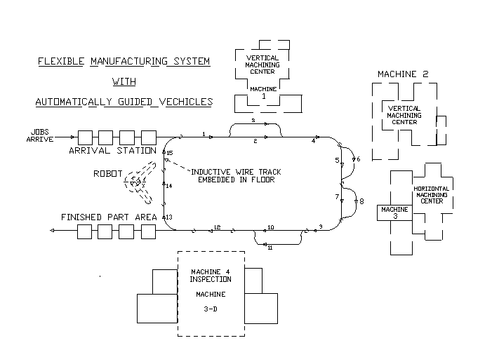
Figure 23—1. The AGV System.
The robot, machine tools, and automatically guided vehicles are controlled by a central computer.
·
Thirty-five percent of components are machined on Machine1.·
Forty-five percent of components are machined on Machine2.·
Twenty percent of components are machined on Machine3.However, 15% of Machine1 jobs and 10% of Machine2 jobs are subsequently machined on Machine3. Jobs consigned originally to machine 3 are machined solely on that machine. Finally, 4% of all components are inspected at random on Machine4.
The wire in the floor guiding vehicles is divided into fifteen 10-meter sections represented by Facilities 1 to 15. The guided vehicles travel at an average speed of 0.5 meters per second, including loading and unloading times.
1. Simulate the operation of the FMS system for 15 days.
2. Determine the utilization of the machine tools.
3. Find the transit time of components through the production system and the in-process storage.
4. Determine the appropriate number of AGVs for the proposed workload in the FMS.
Listing
; GPSS World Sample File - FMSMODEL.GPS, by Gerard F. Cummings
***********************************************************************
*
* AGV Model in FMS Factory *
* *
***********************************************************************
* Time unit is one second
***********************************************************************
* P1 =1 Means machine 1 is req’d first
* P2 =2 Means " 2 " " "
* P3 =3 Means " 3 " " "
***********************************************************************
RMULT 71143
Transit TABLE M1,4000,4000,8 ;Transit time of jobs
Type VARIABLE RN1@16+1 ;Categories of jobs processed
AGV STORAGE 2
*
Inspect FUNCTION P4,L16
1,1200/2,1350/3,1500/4,1650/5,1800/6,1950/7,2100/8,2250/9,2400/10,2550
11,2700/12,2850/13,3000/14,3150/15,3300/16,3450
*
Product FUNCTION P4,L16
1,600/2,700/3,800/4,900/5,1000/6,1100/7,1200/8,1300/9,1400/10,1500
11,1600/12,1700/13,1800/14,1900/15,2000/16,2100
*
Mach1 FUNCTION RN1,D3
.35,1/.80,2/1.0,3
***********************************************************************
GENERATE 720,60
;Xacts are jobs
QUEUE Arrival
;Arrival area queue
ASSIGN 5,FN$Mach1
;P5 is and index to machines
*——Dummy values are put into parameters 1,2, and 3 so that they
*——will be set up to receive the appropriate value
*——in ASSIGN P5,P5.
*——When P1, P2 or P3 are tested in various test Blocks they must
*——already exist.
ASSIGN 1,6
;Dummy value
ASSIGN 2,6
;Dummy value
ASSIGN 3,6
;Dummy value
*——The contents of parameter 5 is put into the parameter with the
*——same number as the contents value(e.g. If parameter 5 has a
*——value of 3, a 3 is put into parameter 3 indicating processing
*——should start on machine 3.
ASSIGN P5,P5
;P1=1, P2=2, or P3=3
ASSIGN 4,V$Type
;P4 = Complexity of job
ENTER AGV
;GET AN AGV
SEIZE Robot
;Get robot
ADVANCE 60
;Time to get an AGV
DEPART Arrival
;Depart arrival queue
ADVANCE 45
;Robot load job on AGV
RELEASE Robot
;Free the robot
SEIZE 1
;Get section 1 of track
ADVANCE 20
;20 second to move 10 M
RELEASE 1
;Free section 1 of track
TEST E P1,1,Skipone
;Machine 1 req’d?
TRANSFER .10,,Next3
;10% also go to Machine 3
First SEIZE 3
;Get section 3 of track
ADVANCE 20
;Move 10 meters
LEAVE AGV
;Free AGV
QUEUE One
;Queue for machine 1
RELEASE 3
;Free section 3 of track
SEIZE Machine1
;Get machine 1
DEPART One
;Depart the queue
ADVANCE FN$Product
;Machining on vertical CNC
RELEASE Machine1
;Machining center
QUEUE Wipone
;Join work-in-progress
ENTER AGV
;Get an AGV
ADVANCE 60
;Time to get an AGV
DEPART Wipone
;Depart work-in-progress
***********************************************************************
Second SEIZE 4
;Get section 4 of track
ADVANCE 20
;10 section to move 10 M
RELEASE 4
;Release section 4
TEST E P2,2,Skiptwo
;Is machine 2 req’d?
TRANSFER .15,,Next4
;15% also go to machine 3
Andthree SEIZE 6
;Get section 6 of track
ADVANCE 20
;Move 10 meters
LEAVE AGV
;Free the AGV
QUEUE Two
;JOIN QUEUE TWO
RELEASE 6
;Free section 6 of track
SEIZE Machine2
;Get machine 2
DEPART Two
;Depart queue 2
ADVANCE FN$Product
;Process on horizontal
RELEASE Machine2
;CNC machining center
QUEUE Wiptwo
;Queue work-in-progress
ENTER AGV
;Get an AGV
ADVANCE 60
;Time to get an AGV
DEPART Wiptwo
;Depart work-in-progress
***********************************************************************
Third TEST E P3,3,Skipthree ;Is machine 3 req’d?
SEIZE 8
;Get section 8 of track
ADVANCE 20
;Move 10 meters
LEAVE AGV
;Free AGV
QUEUE
Three ;Join queue three
RELEASE 8
;Free section 8 of track
SEIZE Machine3
;Get machine 3
DEPART Three
;Depart queue three
ADVANCE FN$Product
;Process on CNC lathe
RELEASE Machine3
;Free turning center
QUEUE Wipthree
;Queue work in progress
ENTER AGV
;Get an AGV
ADVANCE 60
;Time for AGV to arrive
DEPART Wipthree
;Depart work-in-progress
***********************************************************************
Fourth SEIZE 9
;Get section 9 of track
ADVANCE 20
;Move 10 meters
RELEASE 9
;Free section 9 of track
TRANSFER .960,,Skipfour ;4% Of components inspected
SEIZE 11
;Get section 11 of track
ADVANCE 20
;Move 10 meters
LEAVE AGV
;Free the AGV
QUEUE Four
;Join queue four
RELEASE 11
;Free section 11 of track
SEIZE Machine4
;Get Machine 4
DEPART Four
;Depart queue 4
ADVANCE FN$Inspect
;Inspection on 3D machine
RELEASE Machine4
;Release machine 4
QUEUE Wipfour
;Join work-in-progress
ENTER AGV
;Get and AGV
ADVANCE 60
;Time for AGV to arrive
DEPART Wipfour
;Depart work-in-progress
***********************************************************************
Fifth SEIZE 12
;Get section 12 of track
ADVANCE 20
;Move 10 meters
RELEASE 12
;Free section 12 of track
SEIZE Robot
;Get a robot
ADVANCE 45
;Robot unloads job from AGV
RELEASE Robot
;Free the robot
TABULATE Transit
;Record transit time
SAVEVALUE P4+,1
;One job finished
SEIZE 13
;Get section 13 of track
ADVANCE 20
;Recirculate AGV
RELEASE 13
;Free section 13 of track
SEIZE 14
;Get section 14 of track
ADVANCE 20
;Move 10 meters
RELEASE 14
;Free section 14 of track
SEIZE 15
;Get section 15 of track
ADVANCE 20
;Move 10 meters
RELEASE 15
;Free section 15 of track
LEAVE AGV
;Free AGV
TERMINATE
;Destroy xact
***********************************************************************
Next3 ASSIGN 3,3
;10% Use machine 1 and 3
TRANSFER First
Next4 ASSIGN
3,3 ;15% Use machine 2 and 3
TRANSFER ,Andthree
***********************************************************************
Skipone SEIZE 2
;Seize section 2 of track
ADVANCE 20
;Move 10 meters
RELEASE 2
;Free section 2 of track
TRANSFER ,Second
***********************************************************************
Skiptwo SEIZE 5
;Get section 5 of track
ADVANCE 20
;Move 10 meters
RELEASE 5
;Free section 5 of track
TRANSFER ,Third
***********************************************************************
Skipthree SEIZE 7
;Get section 7 of track
ADVANCE 20
;Move 10 meters
RELEASE 7
;Free section 7 of track
TRANSFER ,Fourth
***********************************************************************
Skipfour SEIZE 10
;Get section 10 of track
ADVANCE 20
;Move 10 meters
RELEASE 10
;Free section 10 of track
TRANSFER ,Fifth
***********************************************************************
GENERATE 28800
;Xact every day
TERMINATE 1
;Destroy timer xact
The model is organized into several segments. After the non Block Entities are defined, there are two more model segments. Transactions in the top segment represent jobs, those in the bottom segment time the simulation by decrementing the Termination Count every simulated day.
Transactions representing jobs acquire attributes by passing through ASSIGN Blocks, then serially acquire an AGV, sections of track, a robot, and other production machines, as needed.
Running the Simulation
To run the simulation and create a Standard Report,
CHOOSE File / Open
and in the dialog box
SELECT Fmsmodel
and then
SELECT Open
Next, create the simulation
CHOOSE Command / Create Simulation
then
CHOOSE Command / START
and in the dialog box, replace the 1.
TYPE
15SELECT OK
The simulation will end when 15 transactions have entered the TERMINATE 1 Block. This represents 15 days of operation.
When the simulation ends, GPSS World writes a report to the default report file, FMSModel.1.1. As discussed in Chapter 1, the Report extension will vary depending on saved simulations and previously existing reports. For our purposes, we will assume that this is the first time the simulation has been created and run giving an extension of 1.1.
This report will be automatically displayed in a window. If you close the window, you can reopen it by using the GPSS World File / Open in the Main Menu. Then you should choose Report in the "Files of type" drop down box at the bottom of the window. GPSS World reports are written in a special format. If you wish to edit the report, you will have to copy its contents to the clipboard and from there into a word processor. You will not be able to open the file directly in a word processor.
Discussion of Results
The Standard Report gives the utilizations of the machine tools. Machine2 had the highest utilization (80%).
The distribution of completion times is given in the GPSS Table named Transit. The average completion time was about 3208.1 seconds, with a standard deviation of 1954.9.
Inside the Simulation
Let's now explore the ending condition of the simulation, which generated the Standard Report above. If you are not at the end of the simulation, please translate the model and run it again.
Now, let’s open some graphics windows.
CHOOSE Window / Simulation Window / Storages Window
This is the Storages Window. It gives utilization and queuing information on the AGVs. They encountered a 31% utilization. It would appear that there are sufficient AGVs. Later, we will repeat the simulation using 1 AGV instead of 2.
We’ll look at the histogram for completion times.
CHOOSE Window / Simulation Window / Table Window
and in the drop-down box in the dialog box, TRANSIT is already selected.
SELECT OK
To see the utilizations and queuing statistics for the machine tools press
CHOOSE Window / Simulation Window / Facilities Window
The numbered Facilities represent AGV track segments. If you use the scroll bar to move to the bottom of the window, you will be able to display statistics for the machine tools.
Now, let’s repeat the simulation using a single AGV, but first close up all graphics
windows except the Table Window.CLICK ON The X-Upper Right of Each Window
Next, we’ll redefine the Storage size.
CHOOSE Command / Custom
and in the dialog box
TYPE
AGV Storage 1SELECT OK
Then, we have to clear out the old statistics.
CHOOSE Command / CLEAR
Now, start the simulation, making sure you can observe the Table "Transit" in the Table Window.
CHOOSE Command / START
and in the dialog box, replace the 1.
TYPE
15SELECT OK
This result is a bit surprising! The average completion time went up only slightly when we removed an AGV!
We must be careful—we are certainly not yet justified in reporting that 1 AGV performs close to the way that 2 do. Perhaps we are only observing an effect due to random variation. The GPSS World ANOVA Command is provided to test the significance of results such as these. It is discussed in Lesson 13 of this manual and Chapter 6 of the GPSS World Reference Manual. If this result is sustained, it would appear that the use of 2 AGVs under these circumstances may be an unnecessary luxury.
If you wish to go on to the next lesson, close all windows related to this model.
CLICK ON The X-Upper Right of Each Window
Otherwise, to end the session
CLICK ON The X-Upper Right of Main Window.
Simulation of an Ethernet.
Problem Statement
A 10 Mbps Ethernet network is currently running satisfactorily with 100 workstations online. It has been determined that network traffic is composed of two classes of messages that are generated with the same proportion at all nodes.
The global message arrival pattern in the peak hour can be modeled as a Poisson process, with individual workstations chosen randomly.
We are to determine the effect on performance of adding an additional 100 workstations to the network.
Listing
; GPSS World Sample File - ETHERNET.GPS
***********************************************************************
*
* 10 Mbps Ethernet Model
*
* (c) Copyright 1993, Minuteman Software.
* All Rights Reserved.
*
*
*
* Messages arrive exponentially, as one of two types: short
* or long. A Node is selected and held for the duration of
* message transmission and any collision backoffs.
*
* Each Node on the Ethernet is busy with a single message
* until it is sent, or after some number of collisions (with
* transmission attempts from other nodes) a permanent error
* is declared and the node is released.
*
* Time is in units of milliseconds. Nodes are presumed
* to be 2.5 m. apart. The node ID numbers are used to
* determine the separation distance when calculating
* the collision window. The propagation delay to an adjacent
* node is 0.01 microsecond. Each bit is transmitted in 0.1
* microsecond. The interframe gap is modelled by having the
* sender hold the Ethernet for an additional delay after it
* has sent its message.
*
* Messages are represented by GPSS Transactions. Nodes
* and the Ethernet are represented by GPSS Facilities. An
* additional Facility is used during jamming to prevent the
* startup of any new messages.
*
* A collision results from multiple transmission attempts
* at two or more nodes. The signal propagation delay
* prevents nodes from having simultaneous knowledge of
* each other, thereby leading to this possibility. The time
* interval until the signal from the other node can be
* detected is called the node’s "Collision Window".
*
* Collisions are represented by removing the transmitting
* Transaction from ownership of the Ethernet and sending it
* to a backoff routine. The new owner jams the Ethernet
* briefly and then goes through the backoff, itself. When a
* Transaction’s message is being sent, the transaction has
* ownership of the Ethernet Facility at priority 0, and can
* be PREEMPTed by Transactions which are at priority 1.
* When a Transaction is jamming, it has ownership of the
* Ethernet Facility at priority 1, and is never itself
* PREEMPTed.
*
*
* Arguments:
* 1. Node_Count Number of Nodes 2.5 m. apart
* 2. Min_Msg Bits
* 3. Max_Msg Bits
* 4. Fraction_Short_Msgs Parts per thousand
* 5. Intermessage_Time Global Interarrivals
*
*
***********************************************************************
Node_Count EQU 100 ;Total Ethernet Nodes
Intermessage_Time EQU 1.0 ;Avg. Global Arrival every msec.
Min_Msg EQU 512 ;The Shortest Message in bits
Max_Msg EQU 12144 ;The Longest Message in bits
Fraction_Short_Msgs EQU 600 ;Short Msgs in parts per
thousand
Slot_Time EQU 0.0512 ;512 bit times
Jam_Time EQU 0.0032 ;32 bit times
Backoff_Limit EQU 10 ;No more than 10 backoffs
Interframe_Time EQU 0.0096 ;96 bit times
***********************************************************************
*
* Definitions of GPSS Functions and Variables.
*
***********************************************************************
Backoff_Delay VARIABLE Slot_Time#V$Backrandom ;Calc the
Backoff Delay
Backrandom VARIABLE 1+(RN4@((2^V$Backmin)-1))
Backmin VARIABLE
(10#(10’L’P$Retries))+(P$Retries#(10’GE’P$Retries))
Node_Select VARIABLE 1+(RN3@Node_Count)
Collide VARIABLE
ABS((X$Xmit_Node-P$Node_ID)/100000)’GE’(AC1-X$Xmit_Begin)
Msgtime VARIABLE (0.0001)#V$Msgrand
Msgrand VARIABLE
Min_Msg+(RN1’G’Fraction_Short_Msgs)#(Max_Msg-Min_Msg)
***********************************************************************
*
* The Message Delay Histogram
*
***********************************************************************
Msg_Delays QTABLE Global_Delays,1,1,20
***********************************************************************
*
* Main Body of Model
*
***********************************************************************
*
***********************************************************************
* Message Generation
***********************************************************************
GENERATE (Exponential(1,0,Intermessage_Time)) ;Single msg
; generator
ASSIGN Node_ID,V$Node_Select ;Acquire a Node ID.
ASSIGN Message_Time,V$Msgtime ;Calc and Save XMIT Time.
ASSIGN Retries,0
;No Collisions at start.
***********************************************************************
* Wait for the Node to finish any previous work.
***********************************************************************
QUEUE Global_Delays
;Start timing
SEIZE P$Node_ID
;Wait for, occupy, the Node.
Try_To_Send PRIORITY 1
;Don’t Lose Control
SEIZE Jam
;Wait for any
RELEASE Jam
;Jam to end.
TEST E F$Ethernet,1,Start_Xmit ;If Ethernet Free, jump.
***********************************************************************
*
* The Ethernet is busy. We check to see if we are in the
* Sender’s "Collision Window". If so, this node would
* start transmitting anyway, since the carrier would not
* yet be sensed. In that case, we must initiate a Collision.
*
If Prop Delay to Sender is >= Xmit Time up till now,
* collide.
*
***********************************************************************
TEST E V$Collide,1,Start_Xmit ;No Collision. Go
;Wait for it.
* * * * * * * * * * * * Collision * * * * * * * * * * * * *
Collision PREEMPT Ethernet,PR,Backoff,,RE ;Remove the old owner.
SEIZE Jam
;Jam the Ethernet.
ADVANCE Jam_Time
;Wait the Jam Time.
RELEASE Jam
;End the Jam.
RELEASE Ethernet
;Give up the Ethernet.
PRIORITY 0
;Back to Normal priority.
Backoff ASSIGN Retries+,1 ;Increment the Backoff Ct.
TEST LE P$Retries,Backoff_Limit,Xmit_Error ;Limit
;retries.
ADVANCE V$Backoff_Delay ;Wait to initiate retry.
TRANSFER ,Try_To_Send
;Go try again.
***********************************************************************
* Get the Ethernet, and start sending.
***********************************************************************
Start_Xmit SEIZE Ethernet ;Get Ethernet, wait if
; necessary
SAVEVALUE Xmit_Node,P$Node_ID ;Identify the sender.
SAVEVALUE Xmit_Begin,AC1 ;Mark the start xmit time.
PRIORITY 0
;Ensure we can be PREEMPTed.
ADVANCE P$Message_Time
;Wait until Msg. is sent.
ADVANCE Interframe_Time ;Hold the Ethernet for gap.
RELEASE Ethernet
;Give up the Ethernet.
Free_Node RELEASE P$Node_ID ;Give up the node
DEPART Global_Delays
; to the next msg.
TERMINATE
;Destroy the Message.
***********************************************************************
Xmit_Error SAVEVALUE Error_Count+,1 ;Count the Error.
TRANSFER ,Free_Node
; and get out of the way.
***********************************************************************
*
* Timer Segment
*
***********************************************************************
GENERATE 1000
;Each Start Unit is 1 Second.
TERMINATE 1
*
***********************************************************************
Running the Simulation
To run the simulation and create a Standard Report, in the Model WindowCHOOSE File / Open
and in the dialog box
SELECT Ethernet
and then
SELECT Open
Next, create the simulation
CHOOSE Command / Create Simulation
Now, we open a histogram of message delays,
CHOOSE Window / Simulation Window / Table Window
and in the drop-down box in the dialog box, MSG_DELAYS is already selected.
SELECT OK
Adjust the window so you can see both the Journal Window and the histogram in the Table Window at the same time. O.K. Now, let's do some simulating.
CHOOSE Command / START
and in the dialog box since 1 is the Termination Count we want,
SELECT OK
As the messages pass through the Ethernet, their durations are registered in the Qtable Msg_Delays, and we observe their accumulation in the histogram. The simulation will end when a second of activity has been simulated. From the Table Window we can see that the average message delay time was a little less than 1 millisecond.
When the simulation ends, GPSS World writes a report to the default report file, Ethernet.1.1.
Discussion of Results
Let’s take a look at the report, now. Move down to the utilization of the Facility Entity used to represent the Ethernet. Its utilization was a moderate 48%. Now, look at the entry count for the Block labeled Collision. Apparently, there were only 3 collisions during the simulation. This comes out to 0.003 collisions per message. Go ahead and close the Report Window. You do not have to save the Report Object.
It appears that the network is performing satisfactorily. Now let’s predict the effect of adding 100 more workstations.
Go ahead and close the report.
CLICK ON The X-Upper Right of Report Window.
then,
CLICK ON The Journal Window
make it a comfortable viewing size and
CHOOSE Command / CLEAR
Now, we change the experimental parameters. We’ll do them both in a single Custom Command.
First, the count of workstations.
CHOOSE Command / Custom
TYPE
Node_Count EQU 200PRESS [Enter]
Next, in the second line, the global message interarrival time.
TYPE
Intermessage_Time EQU 1.0#(100/200)SELECT OK
Now, we will simulate the new conditions.
CHOOSE Command / START
and in the dialog box since 1 is the Termination Count we want,
SELECT OK
As you can see in the Table Window, a large proportion of the messages is experiencing delays due to collision backoffs. The average message delay has skyrocketed to over 14 milliseconds.
In a real study, of course, we would simulate much longer, and we would run an Analysis of Variance to establish statistical significance.
Although there is still another step to take from average message delay to performance as perceived by the end user, we would have to conclude that there appear to be serious performance problems in store for this network, if the projected 100 workstations were brought online.
The next step would be to consider, and simulate, the effects of various remedial actions. Let’s look at the report produced after we altered the model.
When the simulation ends, GPSS World writes a report to the default report file, Ethernet.1.1. As discussed in Chapter 1, the Report extension will vary depending on saved simulations and previously existing reports. Since this is the second report, the extension produced by this simulation should be 1.2.
This report will be automatically displayed in a window. If you close the window, you can reopen it by using the GPSS World File / Open in the Main Menu. Then you should choose Report in the "Files of type" drop down box at the bottom of the window. GPSS World reports are written in a special format. If you wish to edit the report, you will have to copy its contents to the clipboard and from there into a word processor. You will not be able to open the file directly in a word processor.
Discussion of Results
Let’s look at statistics in the new Standard Report. To shorten the listing, we only used statistics from the first 10 workstations. The other 190 are similar. We see that the Ethernet utilization has grown to 98%, and that there were 413 collisions in the simulated time. Many of the transactions experienced multiple collisions.
Clearly, the time spent backing off from collisions was a large component of the additional message delay times.
All this information is available in the online Facilities and Blocks Windows. You should open these windows to be sure you can find the information. Look at both detailed view and non-detailed view in these windows.
If you wish to go on to the next lesson, close all windows related to this model.
CLICK ON The X-Upper Right of Each Window
Otherwise, to end the session
CLICK ON The X-Upper Right of Main Window.
Predator-Prey Model.
Problem Statement
A population of rabbits has grown uncontrollably on a small island. The problem is so severe that local farmers expend considerable effort just to break even financially. They want to introduce a population of foxes to bring the situation under control.The problem is to use the Lotka-Volterra predator prey model in PREDATOR.GPS to simulate the phenomenon. What will happen if a population of 80 foxes is released? How many foxes must be released to eradicate the rabbits?
Listing
; GPSS World Sample File - PREDATOR.GPS
******************************************************************
*
* Lotka-Volterra Predator-Prey Model
*
* Operation:
* Plot Foxes and Rabbits: X 12000; Y 0-3000
* START 1
******************************************************************
******************************************************************
*
* Don’t forget to parenthesize the ODEs.
*
******************************************************************
Foxes INTEGRATE (FoxRate())
Rabbits INTEGRATE (RabbitRate())
******************************************************************
*
* The Initial Values
*
******************************************************************
Foxes EQU 80
Rabbits EQU 1000
******************************************************************
*
* The Model Parameters
*
******************************************************************
K_ EQU 0.2000 ;Predator Efficiency
A_ EQU 0.0080 ;Predator Death Rate
B_ EQU 0.0002 ;Foray (Grazing) Factor
C_ EQU 0.0400 ;Prey Birth Rate
******************************************************************
*
* Discrete Simulation Control Segment
*
******************************************************************
GENERATE 10000
TERMINATE 1
PROCEDURE FoxRate() BEGIN
/*******************************************************
Growth Rate for the Fox Population
*******************************************************/
TEMPORARY BirthRate, DeathRate,
TotRate;
/* Limit the Variable, so we can experiment safely. */
IF (Foxes < 0) THEN Foxes = 0;
IF (Foxes > 10e50) THEN Foxes = 10e50 ;
BirthRate = K_ # B_ # Foxes # Rabbits;
DeathRate = A_ # Foxes;
TotRate = BirthRate - DeathRate;
RETURN TotRate;
END;
PROCEDURE RabbitRate() BEGIN
/*******************************************************
Growth Rate for the Rabbit Population
*******************************************************/
TEMPORARY BirthRate, DeathRate,
TotRate;
/* Limit the Variable, so we can experiment safely. */
IF (Rabbits < 0) THEN Rabbits = 0;
IF (Rabbits > 10e50) THEN Rabbits = 10e50 ;
BirthRate = C_ # Rabbits;
DeathRate = B_ # Foxes # Rabbits ;
TotRate = BirthRate - DeathRate;
RETURN TotRate;
END;
In this model, we use single letters followed by underscores to name constants. This ensures that there will be no clashes with PLUS or GPSS keywords. Since PLUS Expressions used outside PLUS Procedures should be parenthesized, the invocations in Operand A of the INTEGRATE Commands are enclosed in outer parentheses.
Running the Simulation
To run the simulation and create a Plot, in the Main Window
CHOOSE File / Open
and in the dialog box
SELECT Predator
and then
SELECT OK
Next, create the simulation
CHOOSE Command / Create Simulation
Now, we set up a Plot of the fox and rabbit populations, to observe the dynamics.
CHOOSE Window / Simulation Window / Plot Window
Then in the Edit Plot Window enter the information as shown, on the next page, in Figure 25--1. You should be looking at a similar dialog box on your screen. We’ll plot the Fox population and Rabbit population on the same plot. Remember to position the mouse pointer at the beginning of each box and click once before you begin to type. Do not press the [Enter] since that is used when all information has been typed in the box. You can, instead, use [Tab] to move from box to box.
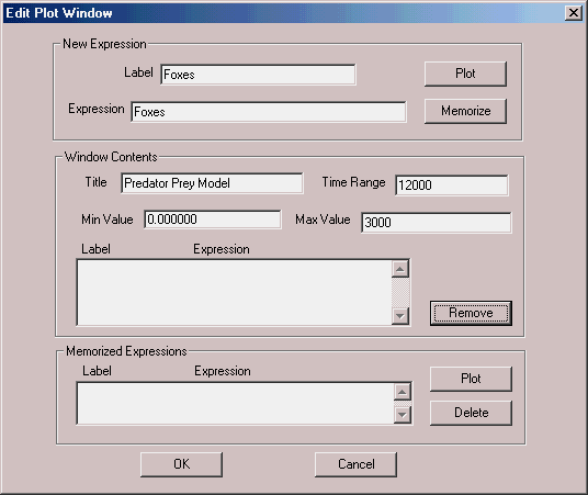
Figure 25—1. The Fox and Rabbit Population Edit Plot Window.
CLICK ON Plot
CLICK ON Memorize
Then enter the Rabbits
Next, to Label, replace the current value
TYPE
Rabbitsand for the Expression, replace the current value
TYPE
Rabbitsand
CLICK ON Plot
CLICK ON Memorize
SELECT OK
Adjust the Plot Window to a comfortable viewing size. Now, let’s get the simulation started.
CHOOSE Command / START
and
SELECT OK
The simulation will end when 10000 time units have passed.
Your Plot Window should look like this:
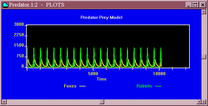
Figure 25—2. Fox and Rabbit Population Dynamics.
Discussion of Results
As you can see, the introduction of foxes causes the rabbit population to decline. Eventually the fox population can no longer be supported, and it too decreases. Eventually there are no longer enough foxes to hold the rabbits in check, and population explosion occurs. With abundant prey, the fox population eventually grows to the point where the rabbits are again under control.
Let’s now determine how many foxes, to the nearest thousand, must be introduced to eliminate the rabbits. Although we could do everything interactively, it’s easy to simply change the starting Fox population and retranslate the model.
Close the Plot Window.
In the Model Window change the Foxes initial value from 80 to 2000.
CHOOSE Command / Retranslate
Now, open a new Plot Window.
CHOOSE Window / Simulation Window / Plot Window
We can set up the plot using the Memorized Expressions. In the Memorized Expressions section of the Edit Plot Window
CHOOSE Foxes
then
CLICK ON Plot
next
CHOOSE Rabbits
and then
CLICK ON Plot
You will have to fill in the information in the Window Contents section of the Edit Plot Window as you did when you set up the first Plot Window.
CHOOSE Command / START
and
SELECT OK
As we can see, during the simulation the populations oscillated even with such a large number of foxes. Let’s try 3000.
Close the Plot Window.
In the Model Window change the Foxes initial value from 2000 to 3000.
CHOOSE Command / Retranslate
Once again, open the Plot Window, as we just did, setting it up in the Edit Plot Window, using the same procedure.
CHOOSE Command / START
and
SELECT OK
After 3 oscillations, the rabbit population died out. With all the prey gone, the fox population also collapsed. Take a look at the values of the Foxes and Rabbits User Variables in the Standard Report. They are both 0.
According to this model, 3000 foxes must be introduced to completely eradicate the rabbits. What happens when 4000 foxes are introduced? Does the system still oscillate?
Inside the Simulation
The integration of ordinary differential equations is sensitive to the conditions you set up. You can expect to be surprised with floating point overflows and the exceeding of error tolerance during the continuous phase, if you haven’t set the derivatives up correctly. In some cases, if you are willing to accept a little less accuracy, you can increase the Integration Tolerance in the Simulation Page of the Model Settings Notebook. Often, you will need to control the variables explicitly. Notice in the predator prey model how the populations are explicitly kept nonnegative in the PLUS Procedures used to evaluate the derivatives.
In practice, differential equations that cause floating point exceptions are often not realistic. Those that are, can usually be replaced by better behaving equivalents that still are able to model the real system.
If you have moved your Plot Window around during this lesson, and discovered that not all the points were redrawn, you can increase the size of the saved point list. To do so, open the Reports Page of the Model Settings Notebook, and type in the new value in the Saved Plot Points entry field.
Now, if you wish to experiment with other models in this tutorial close all windows related to this model.
CLICK ON The X-Upper Right of Each Window
Otherwise, to end the session
CLICK ON The X-Upper Right of Main Window.
We’ve finished with our tutorial lessons. You may find in the future that many of them will serve as good templates for your own models. If you have questions, please don’t hesitate to contact us through our web site.
http://www.minutemansoftware.com