1. TURNSTIL.GPS
Simulation of a turnstile at a football stadium.
Problem Statement
Spectators arrive at a turnstile of a football stadium every 7±7 seconds and queue for admittance. The time to pass through is evenly distributed at 5±3 seconds.
A model is required to determine the time taken by 300 people to pass through the turnstile.
Listing
; GPSS World Sample File - TURNSTIL.GPS, by Gerard F. Cummings
**************************************************************
*
* Turnstile Model
* Time is in seconds
**************************************************************
In_use EQU 5 ;Mean time
Range EQU 3 ;Half range
GENERATE 7,7 ;People arrive
QUEUE Turn
;Enter queue
SEIZE Turn
;Acquire turnstile
DEPART Turn
;Depart the queue
ADVANCE In_use,Range
;Use turnstile
RELEASE Turn
;Leave turnstile
TERMINATE 1
;One spectator enters
**************************************************************
Line by Line Description of Model Function
GENERATE
- The GENERATE Block causes Transactions which represent people to arrive at the turnstile every 7±7 seconds.QUEUE - The QUEUE Block, with the DEPART Block, collect statistics of the waiting line of people who have not yet used the turnstile. The associated GPSS Queue Entity is named Turn.
SEIZE - The SEIZE Block is entered by a single waiting Transaction as soon as the turnstile is available. This causes the turnstile to become busy, thereby preventing any more Transactions from entering the SEIZE Block.
DEPART - Once a Transaction has SEIZEd the Facility representing the turnstile, it enters a DEPART Block in order to collect waiting time statistics for the Queue Entity Turn. The waiting time does not include time in the turnstile.
ADVANCE - The ADVANCE Block controls the length of simulated time that the turnstile is in use by the Transaction that has just SEIZEd it. In this case, the turnstile takes 5±3 seconds to admit a person. We have used named values for the ADVANCE Block operands to make them easy to change as we will see later in this lesson.
RELEASE - The RELEASE Block gives up possession of the turnstile so that a new Transaction can take possession of it by entering the SEIZE Block.
TERMINATE - The TERMINATE Block removes the Transaction from the simulation, after the person has passed through the turnstile.
Running the Simulation
To run the simulation and create a Standard Report, in the Main Window
CHOOSE File / Open
and in the dialog box
SELECT Turnstil
and then
SELECT Open
Next, the simulation must be created.
CHOOSE Command / Create Simulation
then
CHOOSE Command / START
and in the dialog box replace the 1
TYPE 300
and
SELECT OK
The simulation will end when 300 Transactions have entered the TERMINATE Block. This represents 300 people passing through the turnstile.
When the simulation ends, GPSS World writes a report to the default report file, Turnstil.1.1. As discussed in Chapter 1, the Report extension will vary depending on saved simulations and previously existing reports. For our purposes, we will assume that this is the first time the simulation has been created and run giving an extension of 1.1.
This report will be automatically displayed in a window. If you close the window saving the report, you can reopen it by using the GPSS World File / Open in the Main Menu. Then you should choose Report in the "Files of type" drop down box at the bottom of the window. GPSS World reports are written in a special format. If you wish to edit the report, you will have to copy its contents to the clipboard and from there into a word processor. You will not be able to open the file directly in a word processor.
Discussion of Results
From the End Time value in the Standard Report, we see that 2134.023 seconds had elapsed when the 300th spectator had passed through the turnstile. Replications of the simulation will yield slightly different values due to random variation.
Notice that the QUEUE and DEPART Blocks do not enclose the ADVANCE Block. This means that Transactions register waiting time, but not time in the turnstile, in the Queue Entity named Turn. Now look in the Queue Entity subreport of the Standard Report. It is found with QUEUE Turn, above. We see that the maximum number of spectators waiting is 3. That’s not too bad. Perhaps we could get away with a slower turnstile. If spectators arrive, on average, only once every 7 seconds, is it not true that we need only a turnstile that can keep up with arrivals? We’ll find out in a little while.
Inside the Simulation
Let’s now explore the ending condition of the simulation, which generated the Standard Report above. If you are not at the end of the simulation, please Retranslate the model and run it again.
Let’s use the SHOW Command to look at some System Numeric Attributes. Since SNAs are so easy to use, you should be aware of what is available. SNAs are discussed in Chapter 3 of the GPSS World Reference Manual. First, look at the current system clock.
CHOOSE Command / SHOW
and in the dialog box
TYPE AC1
SELECT OK
In the status line of the Main Window you should see the current clock time which is 2134.023.
Next the utilization (fractional busy time) of the turnstile, in parts per thousand.
CHOOSE Command / SHOW
and in the dialog box
TYPE FR$Turn
SELECT OK
This yields a value of 689.67, the Fractional Busy Time is expressed in parts per thousand.
The number of spectators to arrive at the turnstile.
CHOOSE Command / SHOW
and in the dialog box
TYPE N1
SELECT OK
As we expected, it’s 300.
Now, let’s open some graphics windows.
CHOOSE Window / Simulation Window / Facilities Window
This is the Facilities Window. Be sure to expand the window to a comfortable viewing size. Notice that the turnstile was occupied about 70% of the time, and that at the end of the simulation, the turnstile is idle. This is apparent because the Facility representing the turnstile is not busy (gray in color), and no Transaction is currently the owner.
Let’s take a look at where Transactions are.
CHOOSE Window / Simulation Window / Blocks
This is the detailed view of the Blocks Window. Notice that there are no Transactions currently active. That is because Transaction 301 is just about to enter the simulation and Transaction 300 has just been TERMINATEd.
In the detailed view you can see a history of total Block entries during the simulation. This view of the Blocks Window shows the total Block entry counts. In your own simulations you may want to use this form of the Blocks Window to verify that Transactions are going where they should.
Before we go on, let’s close the Blocks Window since we don’t want to have to update extra windows that we are not viewing or planning to view in the immediate future.
CLICK ON The X-Upper Right of the Blocks Window
Now, we will rerun the simulation, viewing the simulation through some other windows. You may also choose to close the Facilities Window at this time. However, we will be utilizing it again in the near future.
Now, let’s get rid of Transactions and reset the statistics accumulators. From the Main Menu
CHOOSE Command / Clear
Let’s begin by setting up an Expression Window.
CHOOSE Window / Simulation Window / Expression Window
Then in the Expression Window
When you enter the value in the second box in the dialog box, you should place the mouse pointer in the small box and click once. Do not press
[Enter] to go from the first to the second box as GPSS World then assumes that all values have been entered. You can instead use [Tab] to move from box to box. Now, in the dialog box for the Label fieldTYPE Number of people
and in the Expression field
TYPE N7
This will let us view the number of spectators that have passed through the turnstile. GPSS World makes data collection extremely easy by providing over 50 automatic variables which describe the state of GPSS entities. The only thing you have to do is spell them correctly!
CLICK ON View
and in this example
CLICK ON Memorize
If we memorize all the expressions, we'll be able to close the window and open it again later with easy retrieval of all the values. Also if you save the simulation the values in the Expression Window will be saved with the simulation if they have been memorized.
Let’s also view the current number of customers waiting to enter the turnstile. In the Expression Window
and in the dialog box for the Label field replace the current value
TYPE Q Content
and in the Expression field, replace the current value
TYPE Q$Turn
CLICK ON View
CLICK ON Memorize
Finally, let’s add a third value to view the average waiting time to get into the turnstile.
In the dialog box for the Label field, replace the current value
TYPE Avg Wait
and in the Expression field, replace the current value
TYPE QT$Turn
CLICK ON View
CLICK ON Memorize
SELECT OK
and
CHOOSE Command / START
and in the dialog box replace the 1
TYPE 25,NP
and
SELECT OK
Did you see the simulation run until 25 customers departed the turnstile? Let’s watch the GPSS Facility that represents the turnstile, but first close the Expression Window since it is best to only have open the windows that you need to watch. Since we have memorized all the Expressions, we can open it again later and easily retrieve the values.
CLICK ON The X-Upper Right of the Expression Window
Now, let's take a look at the Facilities Window. If you have closed it,
CHOOSE Window / Simulation Window / Facilities Window
Otherwise click anywhere on the Facilities Window if it is partially hidden from view. Now, let’s start the simulation running for 25 more Transactions and observe the Facilities Window.
CHOOSE Command / START
and in the dialog box replace the 1
TYPE 25,NP
and
CHOOSE OK
When the simulation completes, close the Facilities Window.
CLICK ON The X-Upper Right of the Facilities Window
Now, let’s see what would happen if the turnstile took, 7±4 seconds, instead of 5±3, to admit a spectator. We’ll use a Custom Command to change the named values that were initially defined in the model.
CHOOSE Command / Custom
and in the dialog box on the first line
TYPE In_use EQU 7
then
PRESS [Enter]
Unlike other dialog boxes, pressing the e key will not process the information entered in the box. Instead it will advance you to the next line where you may enter yet another command to be executed.
TYPE Range EQU 4
and
SELECT OK
If you wish, you can use the SHOW Command to ensure the changes have been made. Let’s test one of the values to see how that works.
CHOOSE Command / SHOW
and in the dialog box
TYPE Range
and
SELECT OK
You should see the value 4 in the Status Line of the Main Window. You'll see it in the Journal Window, as well.
Now let’s see what happens with the new ADVANCE Block.
CHOOSE Command / Clear
SELECT OK
to reset the statistics accumulators and set the simulation startup to the same conditions when we first ran the simulation.
CHOOSE Command / START
and in the dialog box replace the 1
TYPE 300
and
SELECT OK
Please wait for the simulation to end. Now open the Expression Window.
CHOOSE Window / Simulation Window / Expression Window
You should see all three expressions in the Memorized Expressions box
CLICK ON The Expression
and then
CLICK ON View
for each expression. When all three expressions are in the Window Contents box
SELECT OK
Notice that the maximum queue length is quite a bit higher than in the original simulation. Also, the average queuing time is higher. This suggests that the slower turnstile may not be acceptable, even though it could, on average, admit all the spectators.
Before reporting these results, we must establish that they are not due to random noise. Also, we may want to exclude starting conditions from the final statistics using the RESET Command. We could plan a set of experiments, and do an analysis of variance on average queue times based on the two different turnstile rates. The GPSS World ANOVA Command is discussed in Lesson 13 of Chapter 1.
You may stop here or choose to go on to the next model.
If you wish to go on to the next lesson, close all windows related to this model.
CLICK ON The X-Upper Right of Each Window
Otherwise, to end the session
CLICK ON The X-Upper Right of Main Window.
Simulation of a simple telephone system.
Problem Statement
A simple telephone system has two external lines. Calls, which originate externally, arrive every 100±60 seconds. When the line is occupied, the caller redials after 5±1 minutes have elapsed. Call duration is 3±1 minutes. A tabulation of the distribution of the time each caller takes to make a successful call is required. How long will it take for 200 calls to be completed?
Listing
; GPSS World Sample File - TELEPHON.GPS, by Gerard F. Cummings
**************************************************************
*
* Telephone System Model
*
**************************************************************
* Simple Telephone Simulation
* Time Unit is one minute
Sets STORAGE 2
Transit TABLE M1,.5,1,20 ;Transit times
GENERATE 1.667,1 ;Calls arrive
Again GATE SNF Sets,Occupied ;Try for a line
ENTER Sets ;Connect call
ADVANCE 3,1 ;Speak for 3+/-1 min
LEAVE Sets ;Free a line
TABULATE Transit ;Tabulate transit time
TERMINATE 1 ;Remove a Transaction
Occupied ADVANCE 5,1 ;Wait 5 minutes
TRANSFER ,Again ;Try again
**************************************************************
Line by Line Description of Model Function
STORAGE
- The Storage Entity Sets, with total capacity of 2, is set up to represent 2 external telephone lines.TABLE - The Table Transit is defined, so that an on-line histogram of call times can be maintained. Just before a Transaction is TERMINATEd, the "time in simulation" SNA, M1, is tabulated. This represents the duration from when the caller first dialed, until he/she finished talking.
GENERATE - A Transaction that represents a call is created every 100±60 seconds.
GATE - A GATE Block sends a Transaction to the Block Occupied when all lines are busy. This occurs when the Storage Entity Sets is full, and represents a caller who must begin waiting before redialing.
ENTER - If either 0 or 1 unit of storage is in use, a Transaction passes through the GATE Block, and into the ENTER Block, thereby using another storage unit. If all storage units are then in use, no more Transactions will be admitted by the GATE Block. Each Transaction passing into the ENTER Block represents a call which has been successfully connected.
ADVANCE - The Transaction then enters an ADVANCE Block, which simulates a call duration of 180±60 seconds. It will remain in this Block until the simulated time has passed.
LEAVE - When a Transaction enters the LEAVE Block, it makes one unit of the Storage Sets available to other Transactions. This represents a newly available external line.
TABULATE - The TABULATE Block adds a call duration to the histogram of call times collected in Table Transit.
TERMINATE - The TERMINATE Block removes the Transaction from the simulation, after the call has been completed.
ADVANCE - A Transaction comes to the ADVANCE Block labeled Occupied when it tried, and failed, to acquire a unit of storage from the Storage Entity Sets. This represents a caller who must wait before redialing.
TRANSFER - The TRANSFER Block sends each Transaction to the GATE Block labeled Again. There, the Transaction will try again to acquire a storage unit from the Storage Entity Sets. In other words, the caller will redial.
Transactions represent calls begun but not completed. If a new caller finds both lines busy, the GATE Block labeled Again sends it to wait in the ADVANCE Block labeled Occupied for 5 minutes, or so. After the delay, the Transaction jumps back up to the GATE Block to try again. Successful callers pass through the GATE Block, encounter a delay which represents the call, and then leave the simulation.
Notice that the number of phone lines is modeled as a Storage Entity with a capacity of 2. Later, it will be very easy to experiment with the effects of adding more lines.
If a call cannot be completed, the corresponding Transaction waits for 5 simulated minutes in the ADVANCE Block labeled Occupied. The number of Transactions here represents the number of callers waiting to redial.
The TABLE statement will produce detailed information on the duration of call attempts. By tabulating the M1 SNA just before each Transaction is TERMINATEd, we will build a histogram of how long callers took to complete their calls.
Running the Simulation
To run the simulation and create a Standard Report,
CHOOSE File / Open
and in the dialog box,
SELECT Telephon
and then
SELECT Open
Next, the simulation must be created.
CHOOSE Command / Create Simulation
then
CHOOSE Command / START
and in the dialog box replace the 1
TYPE 200
SELECT OK
The simulation will end when 200 Transactions have entered the TERMINATE Block. This represents 200 call completions.
When the simulation ends, GPSS World writes a report to the default report file, Telephon.1.1. As discussed in Chapter 1, the Report extension will vary depending on saved simulations and previously existing reports. For our purposes, we will assume that this is the first time the simulation has been created and run giving an extension of 1.1.
This report will be automatically displayed in a window. If you close the window, you can reopen it by using the GPSS World File / Open in the Main Menu. Then you should choose Report in the "Files of type" drop down box at the bottom of the window. GPSS World reports are written in a special format. If you wish to edit the report, you will have to copy its contents to the clipboard and from there into a word processor. You will not be able to open the file directly in a word processor.
Discussion of Results
From the End Time value in the Standard Report, we see that 359.16 minutes had elapsed when the 200th call had been completed. Replications of the simulation will yield slightly different values due to random variation.
The Table named Transit gives detailed information on how long it took callers to complete their calls. Although most calls were completed in less than 9.5 minutes, many took much longer. Perhaps this would be a source of customer dissatisfaction.
Inside the Simulation
Let us now explore the ending condition of the simulation, which generated the Standard Report above. If you are not at the end of the simulation, please Retranslate the model and run it again. If you have a Report Window open, please close it now.
Let’s use the Expression Window to look at some System Numeric Attributes. First, confirm the simulation end time.
CHOOSE Window / Simulation Window / Expression Window
The Edit Expression Window opens. When you enter the value in the second box in this dialog box, you should place the mouse pointer in the small box and click once. Do not press
[Enter] to go from the first to the second box as GPSS World then assumes that all values have been entered. You can, instead, use [Tab] to move from box to box. Now, in the dialog box for the Label fieldTYPE Time
and in the Expression field
TYPE AC1
This will let us view the current time.
CLICK ON View
and
CLICK ON Memorize
If we memorize all the expressions, we'll be able to close the window and open it again later with easy retrieval of all the values. Also if you save the simulation the values in the Expression Window will be saved with the simulation if they have been memorized. We're going to close this window and reopen it later so please memorize this expression and the ones that follow.
Now, let's look at the utilization (fractional busy time) of the phone lines, in parts per thousand.
In the dialog box for the Label field replace the current value
TYPE Util
and in the Expression field, replace the current value
TYPE SR$Sets
CLICK ON View
CLICK ON Memorize
Finally, let’s add the average time a phone line is held.
In the dialog box for the Label field, replace the current value
TYPE Avg. Call Time
and in the Expression field, replace the current value
TYPE ST$Sets
CLICK ON View
CLICK ON Memorize
SELECT OK
The utilization is expressed in parts per thousand. The lines are utilized at 84% of capacity. Although there is some unused time, the queuing delays may not be acceptable.
Now, close the Expression Window
CLICK ON The X-Upper Right of the Window
Now, let’s open some graphics windows.
CHOOSE Window / Simulation Window / Storages Window
This is the Storages Window Detail View. Notice that we can also see the 84% utilization here. From the low and high water marks (Min and Max values) of the storage in use, we see that some time in the simulation, 0, 1, or 2 lines were busy. Use the slide bar in the bottom of the window to move to the values we are discussing. The Storages Window is discussed in Chapter 5 of the GPSS World Reference Manual.
If we open the Table Window, we can see the histogram of call completion times.
CHOOSE Window / Simulation Window / Table Window
and since there is only one Table in this model you will see TRANSIT in the drop-down box
SELECT OK
Make sure that you size the Table Window so that it is large enough to display the Table correctly. This gives the same information as the Table in the Standard Report. The average talking time is 3 minutes as shown by the ST SNA in the Expression Window, but the average time including redials is 14.27 minutes as seen in the Table Window. Callers are spending an enormous amount of time redialing.
Let’s take a look at where Transactions are.
CHOOSE Window / Simulation Window / Blocks Window
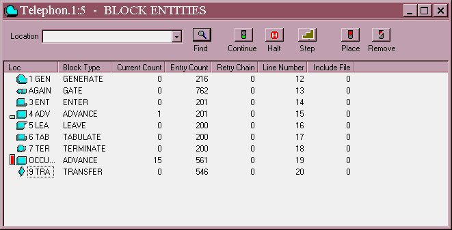
This is the Blocks Window. Notice that 15 customers are waiting to redial.
Look at the history of Block entries in the Entry Count column.
Figure 2—1. Blocks Window Detailed View Showing TRANSFER Block.
What’s going on here? Look at how many Transactions have entered the ADVANCE Block meaning that they are waiting to redial! 561! But there have only been 200 calls. Watch the Blocks Window, and using the Function Key
[F5]. Step through the simulation. Do this 15 or 20 times. Do you see what is happening? Many callers who redial are finding the lines busy, and must wait yet another time to redial.Now we will rerun the simulation, viewing it through some graphics windows. Begin by closing all of the open windows except the Blocks, Journal and Model Windows.
CLICK ON The X-Upper Right of Each Window
Let's reopen the Expression Window with the values that we memorized before and add the call number which is also the Active Transaction number.
CHOOSE Window / Simulation Window / Expression Window
in the Edit Expression dialog box for the Label field
TYPE Call no.
and in the Expression field
TYPE XN1
CLICK ON View
CLICK ON Memorize
Before we open the Window, we need to bring back the memorized Expressions that we entered the first time we opened the Window. For each expression that was memorized in the memorized box
CLICK ON The Expression
then
CLICK ON View
Finally, when all expressions show in the view box
SELECT OK
Now, let’s get rid of Transactions and reset the statistics accumulators. From the Main Menu
CHOOSE Command / Clear
CHOOSE Command / Custom
TYPE RMULT 1
We are resetting Random Number Generator 1 since CLEAR does not do so. This is necessary if you want to ensure the starting point of the stream. In this way, if you've used other commands, not listed in the Tutorial, before the CLEAR, we'll all be seeing the same results during this run. RMULT is discussed in more detail in the ANOVA lesson in Chapter 1.
SELECT OK
In the Blocks Window move the mouse pointer over the last Block in the model which is the TRANSFER Block.
CLICK ON The TRANSFER Block
and
CLICK ON The Place Icon in the Debug Toolbar
Next, size and position the Blocks, Journal and Expression Windows, so you can see each of them.
CHOOSE Command / START
and in the dialog box replace the 1
TYPE 1000,NP
and
SELECT OK
The simulation stops on the first attempt to enter the TRANSFER Block. This indicates that this caller couldn’t get through. Continue the running of the simulation.
PRESS [F2]
Do this same operation four more times after each time the simulation is Halted by the Stop Condition.
The simulation will continue to stop every time a caller has to wait. You will see the trace messages in the Journal Window that indicate the Transaction number of the Stopped Transaction. Since there is only one GENERATE Block in this model, you can see by Transaction number how often a caller is having to wait and if there are callers waiting for a second time.
Now, remove the Stop Condition. In the Blocks Window
CLICK ON The Transfer Block
CLICK ON The Remove Icon in the Debug Toolbar
Then, close the Blocks, and Expression Windows.
CLICK ON The X-Upper Right of Each Window
Now, we’ll watch the simulation run in the Storages Window non-detailed view.
CHOOSE Window / Simulation Window / Storages Window
and from the Main Menu
CHOOSE View / Entity Details
to toggle to the non-detailed view of the window.
Now let’s also watch the call delay histogram as it is being built!
CHOOSE Window / Simulation Window / Table Window
and since there is only one table and its name is already in the drop-down box
SELECT OK
Continue the running of the simulation.
PRESS [F2]
The Table named Transit is, in fact, a dynamic histogram which can be viewed at any time. It shows that many customers are not receiving service right away. Clearly, the customers finding busy lines won’t be too happy. When you have finished watching, close both the Table and Storages Windows and let the simulation run to completion.
What if we added more lines? Let’s simulate 4 lines instead of two.
It’s a good idea use the CLEAR Command before you redefine an entity.
CHOOSE Command / CLEAR
then
CHOOSE Command /Custom
and in the dialog box
TYPE Sets Storage 4
PRESS [Enter]
and on the next line
TYPE RMULT 1
SELECT OK
That redefines the number of phone lines. You can do this with any window open. This action will be recorded in your Journal for later review if you chose to leave it open.
Now, let’s see what happens.
CHOOSE Command / START
and in the dialog box replace the 1
TYPE 1000,NP
and
SELECT OK
The utilization of the phone lines is much smaller as seen in the Storages sectionof the report. Now observe the histogram of call durations.
CHOOSE Window / Simulation Window / Table Window
and since there is only one table and its name is already in the drop-down box
SELECT OK
That’s much better. In fact, if you’d like to look in the detailed view of the Blocks Window, you’ll see that the TRANSFER Block was not entered meaning that no callers had to redial. Four lines appear to be much better than two. This would have to be established statistically, possibly using the ANOVA Command.
We now appear to have a solution to the problem, but it may be unnecessarily expensive. Three phone lines would be less expensive than four, and might suffice. Let’s try it.
CHOOSE Command / CLEAR
then
CHOOSE Command / Custom
and in the dialog box
TYPE Sets Storage 3
to change the number of lines to 3
PRESS [Enter]
and on the next line
TYPE RMULT 1
SELECT OK
Now, let’s see what happens.
CHOOSE Command / START
and in the dialog box replace the 1
TYPE 1000
and
SELECT OK
You may want to open the Blocks Window. When you have observed the open graphics windows as long as you want, close them and let the simulation run to completion. It looks like three phone lines is effective. A quick look at the Report reveals that only 57 callers had to redial. In the Report Window's Table statistics, average transit time is only 3.28 minutes. If the load of calls is not expected to increase, this may be satisfactory.
Before reporting these results, we must prove that they are not due to random noise. Also, we may want to exclude starting conditions from the final statistics using the RESET Command. We could plan a set of experiments, and do an analysis of variance on the average transit times based on the different phone line configurations. Treatment 2 would be the 2 phone line configuration, treatment 3 would have 3 lines, and treatment 4 would have 4 lines. Each simulation should cover several thousand calls, and each treatment level should have several replications using different random number seeds. The GPSS World RESET, and ANOVA Commands are discussed in Chapter 6 of the GPSS World Reference Manual. The ANOVA Command is studied in Lesson 13 of Chapter 1.
You may stop here or choose to go on to the next model.
If you wish to go on to the next lesson, close all windows related to this model.
CLICK ON The X-Upper Right of Each Window
Otherwise, to end the session
CLICK ON The X-Upper Right of Main Window.
Simulation of inventory with periodic review.
Problem Statement
A finished product inventory is controlled by means of a weekly periodic review system. The initial stock is 1000 units. The daily demand varies between 40 and 63 units with equal probability. The target inventory is 1000 units, that is, the order is placed for the difference between the current stock and 1000 units. If the current stock is 800 or more, no order is placed for that week. The company operates a five-day week. The lead time for delivery of an order is one week.
Simulate the inventory system for 200 days and determine if any stockouts occur.
Listing
; GPSS World Sample File - PERIODIC.GPS, by Gerard F. Cummings
***********************************************************************
*
* Periodic Review Inventory Model
* Time units are in days
*
***********************************************************************
* Definitions of non Block entities
RMULT 39941
Stock STORAGE 10000 ;Warehouse can hold 10000
Stock TABLE S$Stock,100,100,20 ;Table for inventory amts
Orderqty VARIABLE Target-S$Stock ;Order quantity
Demand VARIABLE RN1@24+40 ;Daily demand
Target EQU 1000 ;Initial stock level
Reorder EQU 800 ;Reorder point
***********************************************************************
* The reorder process
GENERATE 5,,,,1
;Review xact, Priority=1
TEST L S$Stock,Reorder,Skip ;Is stock < Reorderpt
ASSIGN 2,V$Orderqty ;Parameter 2=Order quantity
Custwait ADVANCE 5
;Lead time is 5 days
ENTER Stock,P2
;Stock increases by P2
Skip TERMINATE
;Ordering xact is finished
***********************************************************************
* The daily demand decrements quantity on hand
GENERATE 1
;Daily demand Transaction
ASSIGN 1,V$Demand
;Parameter 1(P1)=daily demand
TABULATE Stock
;Record daily stock
TEST GE S$Stock,P1,Stockout ;Can order be filled
LEAVE Stock,P1
;Remove demand from stock
TERMINATE 1
;Daily timer
Stockout TERMINATE 1
;Daily timer
***********************************************************************
* Initialize the inventory
GENERATE ,,,1,10
;Set initial stock
ENTER Stock,Target ;Set init stock level=target
TERMINATE
;Xact is terminated
**********************************************************************
Line by Line Description of Model Function
RMULT
- The seed for the random number generator is set. Changing only the seed allows you to measure the effects of purely random variation. Replication simulations form the basis for using the GPSS World ANOVA Command.STORAGE - The Storage Entity Stock is given a capacity of 10000. This is well above the usual levels of inventory, and represents warehouse capacity. We must allow the stock levels to exceed the target level. The Storage content in use will be used to represent the current stock level. Therefore, the current stock level is available throughout the simulation as the SNA S$Stock.
TABLE - A Table, also named Stock, is set up to accumulate a histogram of daily stock levels.
ORDERQTY - The quantity to be ordered is the target stock level, Target, minus the stock on hand.
DEMAND - The daily demand varies from 40 to 63 units, with equal probability. The @ operator denotes modulo arithmetic, reducing a random number between 0 and 999, to one between 0 and 23. The final result is obtained by adding 40. The resulting random numbers will be retrieved via the SNA V$Demand.
TARGET - The target stock level, Target, is set to 1000. The use of a named value makes it easy to experiment with the reorder scheme.
REORDER - The reorder point, Reorder, is set to 800. The use of a named value makes it easy to experiment with the reorder scheme.
We now look at statements which define the Blocks to be entered by Transactions when the simulation is running.
GENERATE - This GENERATE Block creates a Transaction once every 5 simulated days. From here on, we must consistently use one time unit to represent one day. Actually, a high priority initializing Transaction from the last GENERATE Block is active before the first Transaction from this GENERATE Block. A Transaction leaves this Block once every 5 simulated days for the sole purpose of testing the stock level, and reordering only if necessary.
TEST - The TEST Block determines if a reorder is necessary. This occurs if S$Stock is less than Reorder. Otherwise, the entering Transaction skips to Skip, and is destroyed without simulating a reorder.
ASSIGN - If the TEST Block detects the reorder condition, the Transaction passes into the ASSIGN Block. This gives parameter number 2 of that Transaction the quantity to be reordered.
ADVANCE - The Transaction which detects the reorder condition waits for 5 simulated days, to represent the order lead time. Notice that other Transactions are not prevented from ordering.
ENTER - When the simulated order arrives, after 5 simulated days, the Transaction enters the ENTER Block and increases S$Stock by the value in its parameter number 2.
TERMINATE - Transactions are destroyed without decrementing the Termination Count. (The Termination Count is used to specify the simulation’s end condition.)
GENERATE - A Transaction, representing the daily orders, is created once each simulated day.
ASSIGN - The daily demand is placed in parameter number 1 of the Transaction.
TABULATE - The TABULATE Block updates the histogram of daily stock levels, before any orders are filled.
TEST - The TEST Block checks for a stockout. If one is detected, the order is not filled, and we merely send the Transaction to the Block labeled Stockout. Notice that this model only detects stockout conditions without considering their effects. We would have to add more detail to this model, if we were concerned with these effects. Here, however, we will conclude that the ordering scheme is unsatisfactory if there is a single stockout.
LEAVE - If the stock level is sufficient, the Transaction reduces S$Stock by the amount of the daily order. It does so by entering the LEAVE Block specifying parameter number 1 as operand B.
TERMINATE - The Transaction is destroyed, and the Termination Count is reduced by 1, to indicate another day has been simulated.
TERMINATE - The TERMINATE Block labeled Stockout is entered only if a daily Transaction detects that its daily order cannot be satisfied. The simulation does not attempt to model the effects of backorders, or lost orders; it only is designed to detect stockouts. The SNA N$Stockout will return the total number of stockouts detected during the measurement period.
GENERATE - The third GENERATE produces a single Transaction at the beginning of the simulation to initialize the stock level. It has a high priority to ensure that it will not be superseded by other Transactions.
ENTER - The initializing Transaction uses the ENTER Block to set the value of S$Stock to the target level, at the start of the simulation.
TERMINATE - The TERMINATE Block destroys the initializing Transaction without decrementing Termination Count.
Unlike general purpose programming languages, GPSS allows many Transactions to exist at different places in the simulation at any one time. In this model, Transactions are created at each of three GENERATE Blocks, creating three types of Transactions. In the top segment, a Transaction is introduced every 5 business days to review the inventory and reorder, if necessary. After 5 days the order is received and incorporated into the inventory.
In the middle segment Transactions represent the daily demand. They cause items to be removed from inventory if the demand can be filled. Before the demand is been satisfied, the stock level is tabulated in the Table Stock.
The single Transaction created in the last segment sets the initial inventory to 1000 items. This Transaction is given a high priority to ensure that it becomes the first Active Transaction.
Time units are in days. The current content of the Storage Entity named Stock represents the current inventory level. This value is available as the SNA S$Stock. The Table named Stock accumulates a histogram of daily inventory levels.
The named values Target and Reorder represent the two most important parameters of this scheme. Target sets the target stock level and Reorder sets the stock level which triggers a reorder. By using named values, we can easily change these parameters to explore alternate designs.
Running the Simulation
To run the simulation and create a Standard Report,
CHOOSE File / Open
and in the dialog box
SELECT Periodic
and then
SELECT Open
Next, the simulation must be created.
CHOOSE Command / Create Simulation
then
CHOOSE Command / START
and in the dialog box replace the 1
TYPE 200
SELECT OK
The simulation will end when 200 daily orders have been filled.
When the simulation ends, GPSS World writes a report to the default report file, Periodic.1.1. As discussed in Chapter 1, the Report extension will vary depending on saved simulations and previously existing reports. For our purposes, we will assume that this is the first time the simulation has been created and run giving an extension of 1.1.
This report will be automatically displayed in a window. If you close the window, you can reopen it by using the GPSS World File / Open in the Main Menu. Then you should choose Report in the "Files of type" drop down box at the bottom of the window. GPSS World reports are written in a special format. If you wish to edit the report, you will have to copy its contents to the clipboard and from there into a word processor. You will not be able to open the file directly in a word processor.
Discussion of Results
The Table Stock shows that the inventory system satisfied all the daily demands, and never suffered an outage. From the Table Stock in the report, we see that there was never a tabulated daily level less than 300. There may be more efficient systems, but the present one was satisfactory in at least this one respect. Replications of the simulation will yield slightly different values due to random variation.
Inside the Simulation
Let’s now explore the ending condition of the simulation, which generated the Standard Report above. If you are not at the end of the simulation, please Retranslate the model and run it again.
First, let’s set up an Expression Window to view two values now and to use in the future when we wish to add more variables to observe.
CHOOSE Window / Simulation Window / Expression Window
The Edit Expression Window opens. When you enter the value in the second box in this dialog box, you should place the mouse pointer in the small box and click once. Do not press
[Enter] to go from the first to the second box as GPSS World then assumes that all values have been entered. You can, instead, use [Tab] to move from box to box. Now, in the dialog box for the Label fieldTYPE No. Stockouts
and in the Expression field
TYPE N$Stockout
This will let us view stock outages.
CLICK ON View
and
CLICK ON Memorize
If we memorize all the expressions, we'll be able to close the window and open it again later with easy retrieval of all the values. Also if you save the simulation the values in the Expression Window will be saved with the simulation if they have been memorized. We're going to close this window and reopen it later so please memorize this expression and the ones that follow.
Now, let's add the maximum stock level.
In the dialog box for the Label field replace the current value
TYPE Max Stock
and in the Expression field, replace the current value
TYPE SM$Stock
CLICK ON View
CLICK ON Memorize
Now, let's add the current stock level as well.
In the dialog box for the Label field replace the current value
TYPE Stock
and in the Expression field, replace the current value
TYPE S$Stock
CLICK ON ViewCLICK ON Memorize
Finally, let's add the day number.
In the dialog box for the Label field replace the current value
TYPE Day
and in the Expression field, replace the current value
TYPE AC1
CLICK ON View
CLICK ON Memorize
SELECT OK
Our system was successful in preventing outages as seen in the value of the number of stockouts.
The Max Stock shows the most items ever in inventory during the simulation. It appears to be higher than one might expect.
The histogram of daily stock levels is easily available.
CHOOSE Window / Simulation Window / Table Window
and since there is only one table in this model, the name already appears in the drop-down box.
SELECT OK
Notice, that the average stock level is 785.45. This represents money tied up in inventory, and is a measure of the cost of the system.
Let’s continue the simulation, observing the Stock table.
Now, we'll also keep track of the day number as we watch the Expression Window. Next we’ll start the simulation and let it run for 100 days. You may want to make sure that you can see both the Expression Window and the Table Window before you start the simulation running. You can easily do this by resizing the windows.
CHOOSE Command / START
and in the dialog box replace the 1 and use NP to suppress the report.
TYPE 100,NP
and
SELECT OK
That shows data being accumulated during 100 more days of operation.
The internal operation of the simulation is quite simple. At the beginning, the Transaction in the third model segment initializes the Storage Entity Stock. Then, every day a demand Transaction is created in the middle model segment, and every fifth day a reorder Transaction is created in the top model segment. Reorders are not filled for 5 more days.
Close the Tables and Expression Windows.
CLICK ON The X-Upper Right of Each Window
Now, let’s open the Blocks Window in detailed view.
CHOOSE Window / Simulation Window / Blocks Window
This will show total Transaction entry counts.
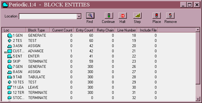
Figure 3—1 The Blocks Window in Detailed View..
We will observe a running history of the simulation.
CHOOSE Command / Clear
and
CHOOSE Command / START
and in the dialog box replace the 1
TYPE 100,NP
and
SELECT OK
Watch the action in the different parts of the simulation by using the slide bar on the right to move around the window. As you can see, there are three different Transaction types. When you have seen enough, halt the simulation if it hasn’t completed.
PRESS [F5]
Perhaps, we could employ a less expensive design with satisfactory results. Open the Table Window.
CHOOSE Window / Simulation Window / Table Window
SELECT OK
Use a Custom Command to change the Target and Reorder levels.
CHOOSE Command / Custom
and in the dialog box
TYPE Target EQU 800
to decrease the target inventory level, and
PRESS [Enter]
and on the next line
TYPE Reorder EQU 600
to decrease the reorder point.
SELECT OK
then
CHOOSE Command / Clear
and
CHOOSE Command / START
and in the dialog box replace the 1
TYPE 100,NP
and
SELECT OK
Please wait for the simulation to end. Put the focus on the Blocks Window and look at the detailed view.
CLICK ON Anyplace on the Blocks Window
Move the slide bar on the right of the window to view the TERMINATE Block labeled Stockout. None occurred. From the Tables Window, we can see the average stock level was lower at 591.420. From our preliminary results, it looks like this is a sufficient, but less costly design.
If you study a long simulation by viewing through the Tables Window, you will see that this inventory control scheme occasionally triggers a second order. This results in an unnecessarily high stock level when both orders have been received. Perhaps a better scheme would adjust a second order when a prior order is outstanding.
Before reporting these results, we must prove that they are not due to random noise. Also, we may want to exclude starting conditions from the final statistics using the RESET Command. We could plan a set of experiments, and do an analysis of variance on the average stock levels based on the different parameters. At the same time we must be aware of the occurrence of outages. The GPSS World RESET, and ANOVA Commands are discussed in Chapter 6 of the GPSS World Reference Manual. The ANOVA Command is studied in Lesson 13 of Chapter 1.
You may stop here or choose to go on to the next model. If you wish to go on to the next lesson, close all windows related to this model.
CLICK ON The X-Upper Right of Each Window
Otherwise, to end the session
CLICK ON The X-Upper Right of Main Window.
Simulation of a television repair shop.
Problem Statement
A television shop employs a single repairman to overhaul its rented television sets, service customers’ sets and do on-the-spot repairs. Overhaul of company owned television sets commences every 40±8 hours and takes 10±1 hours to complete. On-the-spot repairs, such as fuse replacement, tuning and adjustments are done immediately. These arrive every 90±10 minutes and take 15±5 minutes. Customers’ television sets requiring normal service arrive every 5±1 hours and take 120±30 minutes to complete. Normal service of television sets has a higher priority than the overhaul of company owned, rented sets.
1. Simulate the operation of the repair department for 50 days.
2. Determine the utilization of the repairman and the delays in the service to customers.
Listing
; GPSS World Sample File - TVREPAIR.GPS, by Gerard F. Cummings
*****************************************************************
* Television Maintenance Man Model *
*****************************************************************
* Repair of rented sets, one each week *
* Time unit is one minute *
*****************************************************************
GENERATE 2400,480,,,1 ;Overhaul of a rented set
QUEUE Overhaul
;Queue for service
QUEUE Alljobs
;Collect global statistics
SEIZE Maintenance
;Obtain TV repairman
DEPART Overhaul
;Leave queue for man
DEPART Alljobs
;Collect global statistics
ADVANCE 600,60
;Complete job 10+/-1 hours
RELEASE Maintenance
;Free repairman
TERMINATE
;Remove one Transaction
*****************************************************************
* On the spot repairs
GENERATE 90,10,,,3
;On-the-spot repairs
QUEUE Spot
;Queue for spot repairs
QUEUE Alljobs
;Collect global statistics
PREEMPT Maintenance,PR ;Get the TV repairman
DEPART Spot
;Depart the ‘spot’ queue
DEPART Alljobs
;Collect global statistics
ADVANCE 15,5
;Time for tuning/fuse/fault
RETURN Maintenance
;Free maintenance man
TERMINATE
****************************************************************
* Normal repairs on customer owned sets
GENERATE 300,60,,,2
;Normal TV Repairs
QUEUE Service
;Queue for service
QUEUE Alljobs
;Collect global statistics
PREEMPT Maintenance,PR ;Preempt maintenance man
DEPART Service
;Depart the ‘service’ queue
DEPART Alljobs
;Collect global statistics
ADVANCE 120,30
;Normal service time
RETURN Maintenance
;Release the man
TERMINATE
*****************************************************************
GENERATE 480
;One xact each 8 hr. day
TERMINATE 1
* Day counter
*****************************************************************
* Tables of queue statistics
Overhaul QTABLE Overhaul,10,10,20
Spot QTABLE Spot,10,10,20
Service QTABLE Service,10,10,20
Alljobs QTABLE Alljobs,10,10,20
****************************************************************
Line by Line Description of Model Function
GENERATE
- Transactions that represent rental (company owned) sets in need of overhaul are generated, on average, every 40 hours. Time units are minutes. These jobs are given a relatively low priority, of 1.QUEUE - Two QUEUE Blocks are used to keep separate statistics. The QUEUE Block for the Queue Entity Overhaul collects start time statistics for the rental overhaul jobs. The second QUEUE Block for Queue Entity Alljobs is repeated elsewhere in order to capture statistics for the other two job types, as well as this one.
SEIZE - Overhaul jobs wait for, and acquire, a TV repairman represented by the GPSS Facility Entity Maintenance.
DEPART - When an overhaul job Transaction receives ownership of the repairman facility, the waiting time is complete. The two DEPART Blocks register the waiting time in two separate Queue entities.
ADVANCE - This Block simulates the overhaul time to be 600 ±60 minutes.
RELEASE - When an overhaul job is complete, the Transaction representing it gives up ownership of the GPSS Facility Entity representing the TV repairman. This allows another overhaul job to begin.
TERMINATE - The Transaction representing the overhaul job is destroyed, but the Termination Count is not decremented.
GENERATE - Transactions which represent on-the-spot repair jobs are created, on average, every 90 minutes. They have higher priority than the overhaul jobs.
QUEUE - Two QUEUE Blocks are used to keep separate statistics. The QUEUE Block for the Queue Entity Spot collects start time statistics for the on-the-spot jobs. The QUEUE Block for Queue Entity Alljobs is repeated elsewhere in order to capture statistics for the other two job types, as well as this one.
PREEMPT - Since on-the-spot jobs can interrupt the other two job types, Transactions which represent on-the-spot jobs attempt to enter a priority mode PREEMPT Block in order to acquire the repairman. This will temporarily displace any overhaul or normal job Transaction.
DEPART - When an on-the-spot job Transaction receives ownership of the repairman Facility, the waiting time is complete. The two DEPART Blocks register the waiting time in two separate Queue entities.
ADVANCE - The ADVANCE Block simulates the repair time to be 15±5 minutes.
RELEASE - An on-the-spot repair job is complete, the Transaction representing it gives up ownership of the GPSS Facility Entity representing the TV repairman. This allows another job to begin.
TERMINATE - The Transaction representing the on-the-spot job is destroyed, but the Termination Count is not decremented.
GENERATE-TERMINATE - This segment of the model operates in the same way as the last. There is one difference. Whereas on-the-spot jobs can interrupt either normal jobs or overhauls, normal jobs can interrupt only overhauls. Therefore, we give Transactions representing normal jobs a priority (2) between those of the other two job types.
GENERATE - A Transaction, used to count off one day, is created once every 8 simulated hours.
TERMINATE - The counting Transaction is destroyed immediately. This subtracts 1 from the Termination Count, and allows us to control the length of the simulation using operand A of the START Command.
QTABLE - The QTABLE statements, starting with Overhaul, define histograms of the queuing statistics each for display in a Table Window, and to be automatically reported in the Standard Report. We do not need to insert TABULATE Blocks for Qtables because statistics are registered automatically when an associated DEPART Block is entered.
The model is organized into several segments. Each segment has a different type of Transaction. The top three segments represent overhaul, on-the-spot, and normal jobs respectively. All compete for the single Facility Entity, named Maintenance, which represents the repair man. The overhaul jobs are given a lower priority than the others.
The bottom segment times the simulation by causing a Transaction to be created and destroyed once each simulated day. The TERMINATE Block is the only one to decrement the Termination Count provided in the START Command, ending the simulation when the Termination Count (TG1) drops to 0 or below..
The waiting times for each type of job are accumulated by the Queue entities named Overhaul, Spot, and Service. All job delay times are accumulated by the Queue Entity Alljobs. These times do not include the repair time of the jobs, only the delay until the jobs are started.
Qtable entities have been defined for each Queue Entity. This is an easy way to get an automatic histogram of waiting times for each category.
Running the Simulation
To run the simulation and create a Standard Report,
CHOOSE File / Open
and in the dialog box
SELECT TVrepair
and then
SELECT Open
Next, the simulation must be created.
CHOOSE Command / Create Simulation
then
CHOOSE Command / START
and in the dialog box replace the 1
TYPE 50
SELECT OK
The simulation will end after 50 Transactions have entered the TERMINATE Block. This represents 50 days of activity.
When the simulation ends, GPSS World writes a report to the default report file, TVRepair.1.1. As discussed in Chapter 1, the Report extension will vary depending on saved simulations and previously existing reports. For our purposes, we will assume that this is the first time the simulation has been created and run giving an extension of 1.1.
This report will be automatically displayed in a window. If you close the window, you can reopen it by using the GPSS World File / Open in the Main Menu. Then you should choose Report in the "Files of type" drop down box at the bottom of the window. GPSS World reports are written in a special format. If you wish to edit the report, you will have to copy its contents to the clipboard and from there into a word processor. You will not be able to open the file directly in a word processor.
Discussion of Results
We see that the repairman was quite busy, with a utilization of 78%. The average waiting times, to the start of the repair, were 25 for overhaul jobs, and 51 for normal service jobs. There was never a delay in starting an on-the-spot job. The overall average waiting time was about 12 minutes. The waiting times do not include the service times because of our placement of the DEPART Blocks.
Inside the Simulation
Let us now explore the ending condition of the simulation, which generated the Standard Report above. If you are not at the end of the simulation, please Retranslate the model and run it again.
First, confirm the utilization of the repairman. From the menu in the Model Window.
CHOOSE Command / SHOW
and in the dialog box
TYPE FR$Maintenance
SELECT OK
The utilization that you see in the Status line of the Main Window for this SNA is expressed in parts per thousand. It was 78%.
To look at the state of the Facility which represents the repairman, open the Facilities Window.
CHOOSE Window / Simulation Window / Facilities Window
We’re now looking at the detailed view of this window. The average repair time was about 53 minutes.
If we open the Table Window for the Overhaul Table, we can see the histogram of job wait times.
CHOOSE Window / Simulation Window / Table Window
and in the drop-down dialog box,
CLICK ON The Down Arrow
and
SELECT OVERHAUL
SELECT OK
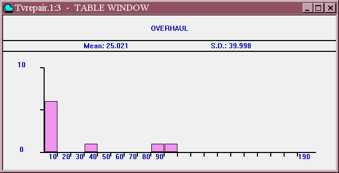
Figure 4—1. The Overhaul Table.
This gives the same information as the Overhaul Table in the Standard Report. To view the other Qtable entities, repeat the action above but choose the names, SERVICE, SPOT or ALLJOBS from the drop-down box. We’ll leave you to look at those on your own. Now close the graphics windows that you have opened.
CLICK ON The X-Upper Right of Each Window
Let’s see what happens when normal jobs arrive every 30 minutes. In the Model Window find the third GENERATE Block (in the normal repairs section of the model). Change it so that operands A and B are 30 and 5 replacing the operands 300 and 60. To do this you simply have to position the mouse pointer at the start of the 300.
CLICK and DRAG The Mouse Pointer Over the 300
and after you release the mouse
TYPE 30
The 300 will be replaced by the 30. Repeat this procedure to change the 60 to 5. Now, Retranslate the model.
CHOOSE Command / Retranslate
Let’s set up a Plot before we run the simulation again.
CHOOSE Window / Simulation Window / Plot Window
Then in the Edit Plot Window enter the information as shown below. You should be looking at a similar dialog box on your screen to the one shown below. We’ll plot the service queue and the utilization of the maintenance man on the same plot. Remember to position the mouse pointer at the beginning of each box and click once before you begin to type. You can, instead, use
[Tab] to move from box to box. Do not press the [Enter] since that is used when all information has been typed in the box.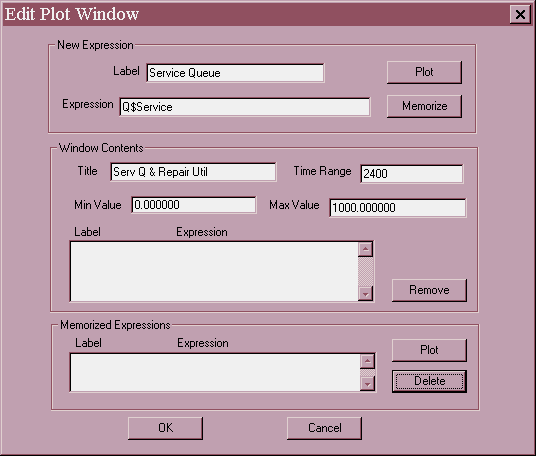
Figure 4—2. The Edit Plot Window
.
CLICK ON
PlotCLICK ON Memorize
Then enter the second set of values we wish to plot
Next to Label replace the current value
TYPE Maintenance Util
and for the Expression replace the current value
TYPE FR$Maintenance
CLICK ON
PlotCLICK ON Memorize
and
SELECT OK
Increase the window to a comfortable viewing size. Now start the simulation.
CHOOSE Command / START
and in the dialog box, replace the 1
TYPE 5,NP
and
SELECT OK
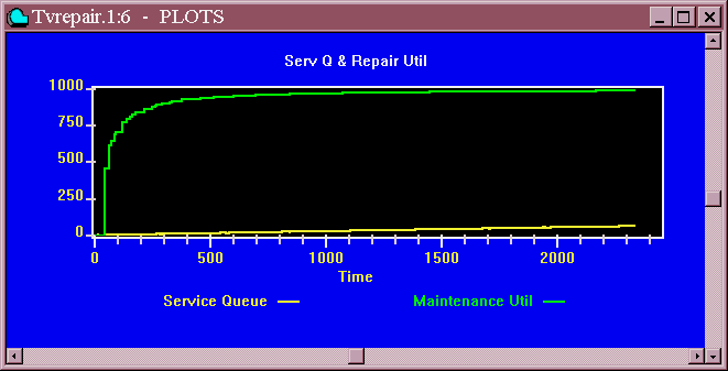
Figure 4—3. Plot of Queue and Utilization.
Clearly the shop is becoming congested and the repairman is working non-stop. Let’s look at one last window. Now close the Plot Window and open the Facilities Window.
CLICK ON The X-Upper Right of Plot Window
and
CHOOSE Window / Simulation Window / Facilities Window
This window confirms the utilization that we just saw and the icon shows a large queue of waiting jobs—62 to be exact. Next,
CHOOSE Window / Simulation Window / Table Window
for each table that you wish to see and choose the appropriate Table name of ALLJOBS, OVERHALL, SERVICE or SPOT from the drop-down box when it appears.
The repairman would certainly need help if jobs came in this fast. Otherwise, the repair shop will probably lose a lot of business.
You may stop here or choose to go on to the next model.
If you wish to go on to the next lesson, close all windows related to this model.
CLICK ON The X-Upper Right of Each Window
Otherwise, to end the session
CLICK ON The X-Upper Right of Main Window.
Simulation of a quality control system.
Problem Statement
A component is manufactured by a sequence of three processes, each followed by a short two minute inspection. The first process requires 20% of components to be reworked. The second and third processes require 15% and 5% of components reworked, respectively. Sixty percent of components reworked are scrapped and the remaining forty percent need reprocessing on the process from which they were rejected.
Manufacturing of a new component commences on average, every 30 minutes, exponentially distributed. The time for the first process is given by the following table.
Time For First Process
Frequency
.05 .13 .16 .22 .29 .15The second process takes 15±6 minutes and the final process time is normally distributed with a mean of 24 minutes and a standard deviation of 4 minutes.
1. Simulate the manufacturing processes for 100 completed components.
2. Determine the time taken, and the number of components rejected.
Listing
; GPSS World Sample File - QCONTROL.GPS, by Gerard F. Cummings
*****************************************************************
* *
* Quality Control Program *
* *
*****************************************************************
RMULT 93211
* Definitions
Transit TABLE M1,100,100,20 ;Transit Time
Process FUNCTION RN1,D7
0,0/.05,10/.18,14/.34,21/.56,32/.85,38/1.0,45
*****************************************************************
GENERATE (Exponential(1,0,30))
ASSIGN 1,FN$Process
;Process time in P1
Stage1 SEIZE Machine1
ADVANCE P1
;Process 1
RELEASE Machine1
ADVANCE 2
;Inspection
TRANSFER .200,,Rework1
;20% Need rework
*****************************************************************
Stage2 SEIZE Machine2
ADVANCE 15,6
;Process 2
RELEASE Machine2
ADVANCE 2
;Inspection
TRANSFER .150,,Rework2
;15% Need rework
*****************************************************************
Stage3 SEIZE Machine3
ADVANCE (Normal(1,24,4)) ;Process 3
RELEASE Machine3
ADVANCE 2
;Inspection 3
TRANSFER .050,,Rework3
;5% need rework
TABULATE Transit
;Record transit time
TERMINATE 1
*****************************************************************
Rework1 TRANSFER .400,,Stage1
TERMINATE
Rework2 TRANSFER .400,,Stage2
TERMINATE
Rework3 TRANSFER .400,,Stage3
TERMINATE
Line by Line Description of Model Function
RMULT
- This sets the seed of random number generator number 1. When we do replication runs, we vary only the random number seeds.TABLE - The Table Transit will accumulate data for a histogram which can be viewed on-line.
FUNCTION - The GPSS function named PROCESS returns a value of 10, 14, 21, 32, 38, or 45, according to the specified probabilities. Notice that in GPSS Functions, you must use Cumulative Distribution Functions to specify probabilities.
GENERATE - New components are started every 30 minutes, on average, exponentially distributed. Here the built-in Exponential distribution is used. Chapter 8 of the GPSS World Reference Manual discusses the built-in distributions.
ASSIGN - The process time for stage one of the job is placed in Transaction parameter number 1.
SEIZE - The job acquires, or waits for, the GPSS Facility Entity named Machine1.
ADVANCE - The job keeps Machine1 busy for the time duration stored in parameter 1 of the Transaction representing the job.
RELEASE - The Transaction representing the job gives up Machine1, which can then be acquired by a waiting Transaction, if there is one.
ADVANCE - The ADVANCE Block simulates the inspection time.
TRANSFER - The TRANSFER Block will randomly select 20% of the Transactions to go to the GPSS Block labeled Rework1. This represents a failure of the part resulting from Stage1. The other 80% of the Transactions go on to the next stage.
SEIZE - The Transaction, which has just passed inspection, acquires, or waits for, the GPSS Facility Entity named Machine2.
ADVANCE - The ADVANCE Block represents the process time for stage 2.
RELEASE - The Transaction representing the job gives up Machine2, which can then be acquired by a waiting Transaction, if there is one.
ADVANCE - The ADVANCE Block simulates the inspection time.
TRANSFER - The TRANSFER Block will randomly select 15% of the Transactions to go to the GPSS Block labeled Rework2. This represents a failure of the part resulting from stage 2. The other 85% of the Transactions go on to the next stage.
SEIZE - The Transaction, which has just passed inspection, acquires, or waits for, the GPSS Facility Entity named Machine3.
ADVANCE - The ADVANCE Block represents the process time for stage 3. The duration is normally distributed.
RELEASE - The Transaction representing the job gives up Machine3, which can then be acquired by a waiting Transaction, if there is one.
ADVANCE - The ADVANCE Block simulates the inspection time.
TRANSFER - The TRANSFER Block will randomly select 5% of the Transactions to go to the GPSS Block labeled Rework3. This represents a failure of the part resulting from stage 3. The other 95% of the Transactions represent completed parts.
TABULATE - The TABULATE Block incorporates a completion time into the histogram associated with the Table named Transit. Tables are written automatically to the Standard Report, and are visible as histograms in the individual Table Windows.
TERMINATE - The TERMINATE Block destroys the Transaction, and decrements the Termination Count. We can simulate a specific number of completed parts by using a part count in operand A of the START statement.
TRANSFER - When a Transaction fails the Stage1 part inspection, it has a 40% probability of being sent back to Stage1. This represents a reworked part.
TERMINATE - The remaining Transactions are destroyed without decrementing the completed part count. This represents scrapping of the parts.
TRANSFER - When a Transaction fails the stage 2 part inspection, and is sent to this TRANSFER Block, it has a 40% probability of being sent back to stage 2. This represents a reworked part.
TERMINATE - The remaining Transactions are destroyed without decrementing the completed part count. This represents scrapping of these parts.
TRANSFER - When a Transaction fails the stage 3 part inspection, it has a 40% probability of being sent back to stage 3. This represents a reworked part.
TERMINATE - The remaining Transactions are destroyed without decrementing the completed part count. This represents scrapping of these parts.
The model is organized into several segments. After the Transit Table, and Process Function are defined, there are three model segments, each representing the corresponding manufacturing process. Each Transaction represents a component in some stage of completion. Time units are in minutes. Each step has a probability of failure, in which case the Transaction is sent to the Block labeled Rework1, Rework2, or Rework3, respectively. Reworked items have a 60% probability of being scrapped. Otherwise they repeat their last step.
Running the Simulation
To run the simulation and create a Standard Report,
CHOOSE File / Open
and in the dialog box
SELECT Qcontrol
and then
SELECT Open
Next, the simulation must be created.
CHOOSE Command / Create Simulation
then
CHOOSE Command / START
and in the dialog box replace the 1
TYPE 100
SELECT OK
The simulation will end when 100 Transactions have entered the TERMINATE Block. This represents 100 completed components.
When the simulation ends, GPSS World writes a report to the default report file, QControl.1.1. As discussed in Chapter 1, the Report extension will vary depending on saved simulations and previously existing reports. For our purposes, we will assume that this is the first time the simulation has been created and run giving an extension of 1.1.
This report will be automatically displayed in a window. If you close the window, you can reopen it by using the GPSS World File / Open in the Main Menu. Then you should choose Report in the "Files of type" drop down box at the bottom of the window. GPSS World reports are written in a special format. If you wish to edit the report, you will have to copy its contents to the clipboard and from there into a word processor. You will not be able to open the file directly in a word processor.
Discussion of Results
From the End Time in the Standard Report, we see that it took 4153.8 minutes or about 69 hours to complete 100 components.
From the Block entry counts, we can derive the number of rejected components. The total entries into Blocks Rework1, Rework2 and Rework3 show that 22 components failed in Stage1, 14 in stage 2 and 4 in stage 3. This is a total of 40 failures. Of these, 21 were scrapped (11+7+3)
Inside the Simulation
Let’s now explore the ending condition of the simulation, which generated the Standard Report above. If you are not at the end of the simulation, please Retranslate the model and run it again.
Let’s use the SHOW Command to look at some System Numeric Attributes. First, confirm the simulation end time.
CHOOSE Command / SHOW
and in the dialog box
TYPE AC1
SELECT OK
In the Status Line, you’ll see that the current time is equal to the end time in the report above.
CHOOSE Command / SHOW
and in the dialog box
TYPE N$Rework1
SELECT OK
This value (22), again is the number of components failing in Stage1.
Now, let’s open some graphics windows.
CHOOSE Window / Simulation Window / Facilities Window
This is the Facilities Window. Notice that the utilization of Machine1 in extremely high, and that there is a large backlog of waiting components. It appears that the failure rate at machine 1 is quite serious, since it is overloading a heavily utilized resource.
The Table Transit is a histogram of completion times. Let’s look at it.
CHOOSE Window / Simulation Window / Table Window
and in the drop-down box you will see TRANSIT since it is the only Table in the model.
SELECT OK
Although the average completion time was 321 minutes, some components took over 800 minutes!
Before going on, close the Facilities and Table Windows.
CLICK ON The X-Upper Right of Each Window
Let’s see where components are. The Blocks Window will give us this information.
CHOOSE Window / Simulation Window / Blocks Window
Notice that 30 components are waiting for Machine1 in the ASSIGN Block. Now, we will rerun the simulation, viewing the simulation through some of the graphics windows. Let’s begin by opening the Expression Window and loading it with some values that we wish to observe.
Let’s keep open the Blocks Window to view the flow the simulation in just a moment. Let’s also open an Expression Window for a view of selected values while the simulation runs.
CHOOSE Window / Simulation Window / Expression Window
Then in the Edit Expression Window for the Label field
TYPE Rework1
And in the Expression field position the mouse pointer anywhere in the Expression box and click once.
TYPE N$Rework1
When we view the Window, this will show us how many parts were sent to possibly be reworked. Remember, a portion of them will just be scrapped.
CLICK ON View
CLICK ON Memorize
Next, look at rework after processing by the second machine. In the Edit Expression Window
in the dialog box for the Label field replace the current value
TYPE Rework2
and in the Expression field replace the current value
TYPE N$Rework2
CLICK ON View
CLICK ON Memorize
Finally, look at rework after processing by the third machine. In the Expression Window
and in the dialog box for the Label field replace the current value
TYPE Rework3
and in the Expression field replace the current value
TYPE N$Rework3
CLICK ON View
CLICK ON Memorize
This will let us view the failing components. Also, in the Blocks Window, we will see failed Transactions entering Blocks Rework1, Rework2 and Rework3.
Let’s also view the component number of the Active Transaction.
In the dialog box for the Label field replace the current value
TYPE Part number
and in the Expression field replace the current value
TYPE XN1
CLICK ON View
CLICK ON Memorize
SELECT OK
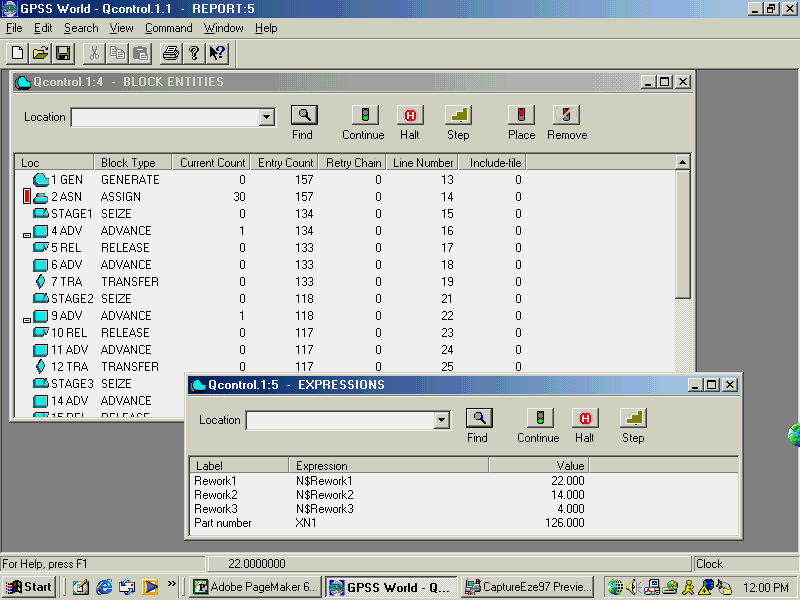
Figure 5—1. Blocks and Expression Windows displayed together.
Now, let’s run the simulation until 50 more components have been completed.
Get ready to watch for reworked components. You may have to size and manipulate the windows to see all the values. Make the Blocks Window active by clicking on it and hide the top of the Expression Window behind it.
CHOOSE Command / START
and in the dialog box replace the 1
TYPE 100,NP
and
SELECT OK
Observe the windows until you see transactions building up in Block 2, The ASSIGN block. This shows that Stage1 in constantly busy and new components as well as those waiting to be reworked are waiting to get into Stage1. As you can see, from looking at the Rework TRANSFER blocks, most components do not fail. Let’s stop the simulation when the next component fails in Stage1. Halt the simulation.
PRESS [F4]
In the detailed view of the Blocks Window, move the mouse pointer over the Block labeled Rework1. You may have to increase the size of the Loc column in the Blocks Window to see the full label as well as increasine the size of the Blocks Window to see both the Stage1 SEIZE block and the Rework1 TRANSFER block.
CLICK ON The Block
then in the Blocks Window
CLICK ON The Place Icon in the Debug Toolbar
Now, continue running the simulation.
PRESS [F2]
The simulation stops when the next Transaction fails in Stage1. It is in the TRANSFER Block, ready to enter the Block labeled Rework1. Now Step the Transaction twice.
PRESS [F5]
twice. If you didn’t see it move, it’s because it wasn’t scrapped, but couldn’t get into Stage1 which is currently busy. It is really on the Delay Chain of the Facility, Machine1. Let’s see how much a lower failure rate in Stage 1 will help the situation. First, close the Blocks Window.
CLICK ON The X-Upper Right of Blocks Window
Remove the Stop from the Rework1 Block
CHOOSE Window / Simulation Snapshot / User Stops
CLICK ON 20
CLICK ON Remove
SELECT OK
Give the Model Window the focus. In the Transfer Block located just above the Block labeled Stage 2, change the failure rate from .200 to .020.
CHOOSE Search / Go To Line
and in the dialog box
TYPE 19
SELECT OK
Now, change the failure rate by replacing the value.
CLICK AND DRAG The Mouse Pointer Over .200
This will highlight this value. Then you can replace it.
TYPE .020
Now, Retranslate the model to incorporate this change.
CHOOSE Command / Retranslate
Now, let’s run it one more time and see how the change affects our factory.
CHOOSE Command / START
and in the dialog box replace the 1
TYPE 100,NP
and
SELECT OK
When the simulation ends, check the end time.
CHOOSE Command / SHOW
and in the dialog box
TYPE AC1
SELECT OK
The end time is 3971.49. The original end time when the failure rate was .200 was 4153.89. It appears that the 100 acceptable parts are being made in a shorter time. Look at the Facilities Window
CHOOSE Window / Simulation Window / Facilities Window
We still have a problem. Machine1 still has a considerable backup even though there has been some improvement. Perhaps we need two machines in the first stage.
Before reporting these results, we must prove that they are not due to random noise. Also, we may want to exclude starting conditions from the final statistics using the RESET Command. We should also be aware that the run time of the simulation we were just examining was extremely short. Longer run times are definitely recommended. We could plan a set of experiments, and do an analysis of variance on the average transit times based on the different failure rates. At the same time we must be aware of the occurrence of outages. The GPSS World ANOVA Command is discussed in Lesson 13 of this manual and in Chapter 6 of the GPSS World Reference Manual
You may stop here or choose to go on to the next model.
If you wish to go on to the next lesson, close all windows related to this model.
CLICK ON The X-Upper Right of Each Window
Otherwise, to end the session
CLICK ON The X-Upper Right of Main Window.